Bill Aging Reports: Part 3/5
Learn how to create, customize, and format pivot tables in Excel for bill review, client filtering, and data analysis. Follow this step-by-step tutorial to efficiently organize and present your data.
In this guide, we'll learn how to create and organize pivot tables to review billing data across different clients and groups. We will cover how to select the right fields for columns, rows, and values, how to filter data for specific clients, and how to format your tables for clarity. This process will help you analyze and present your data more effectively.
Let's get started
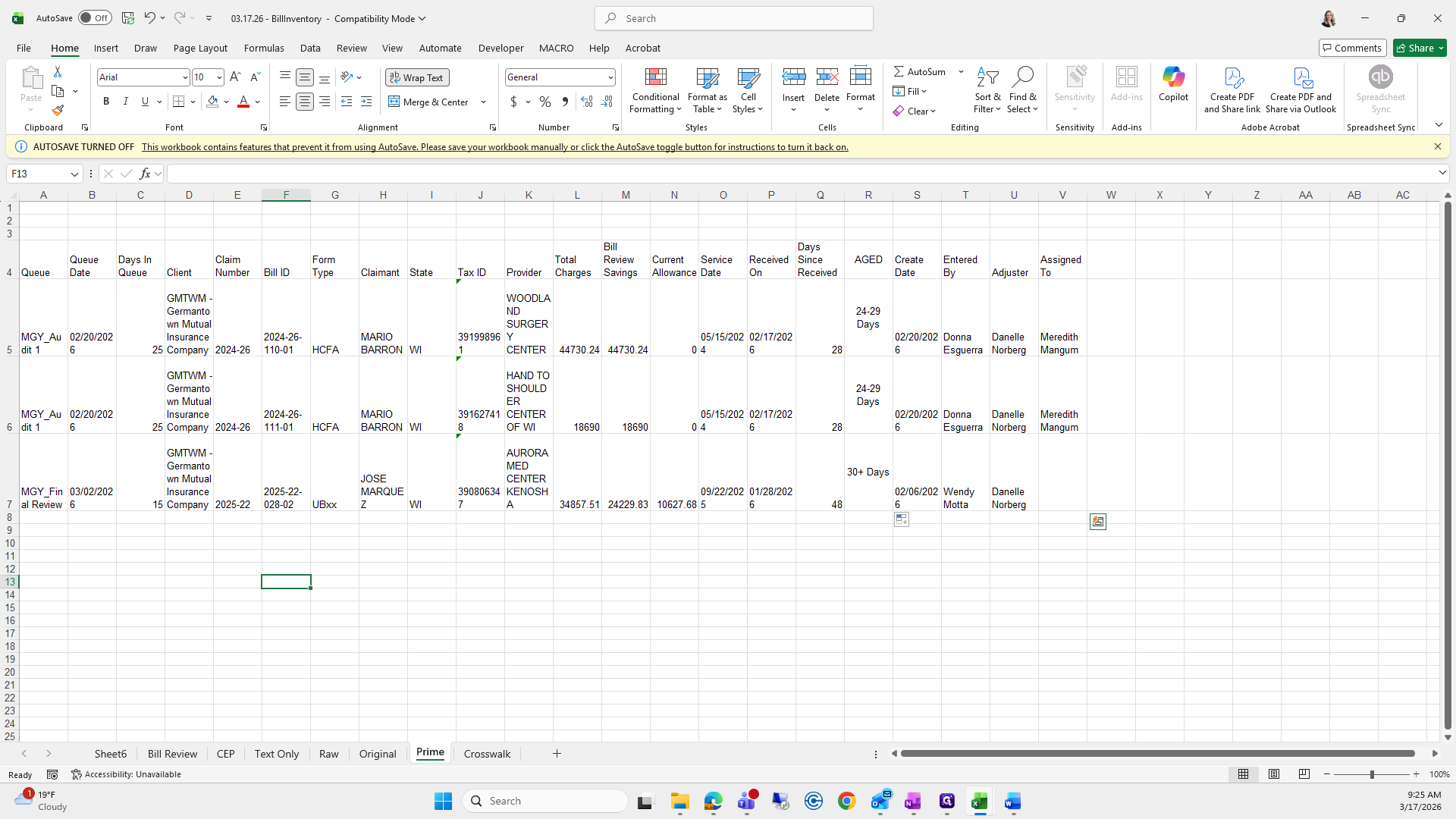
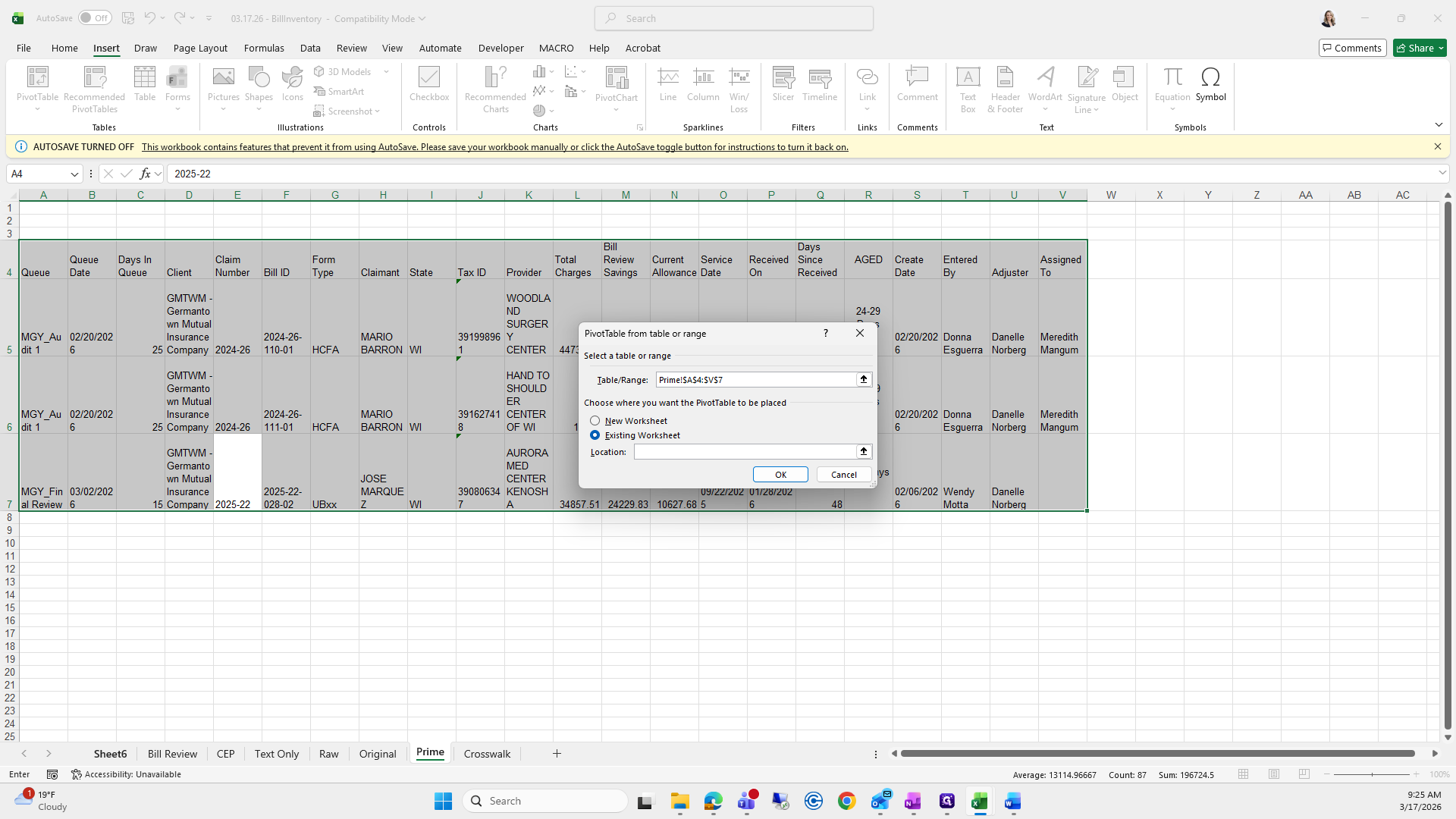
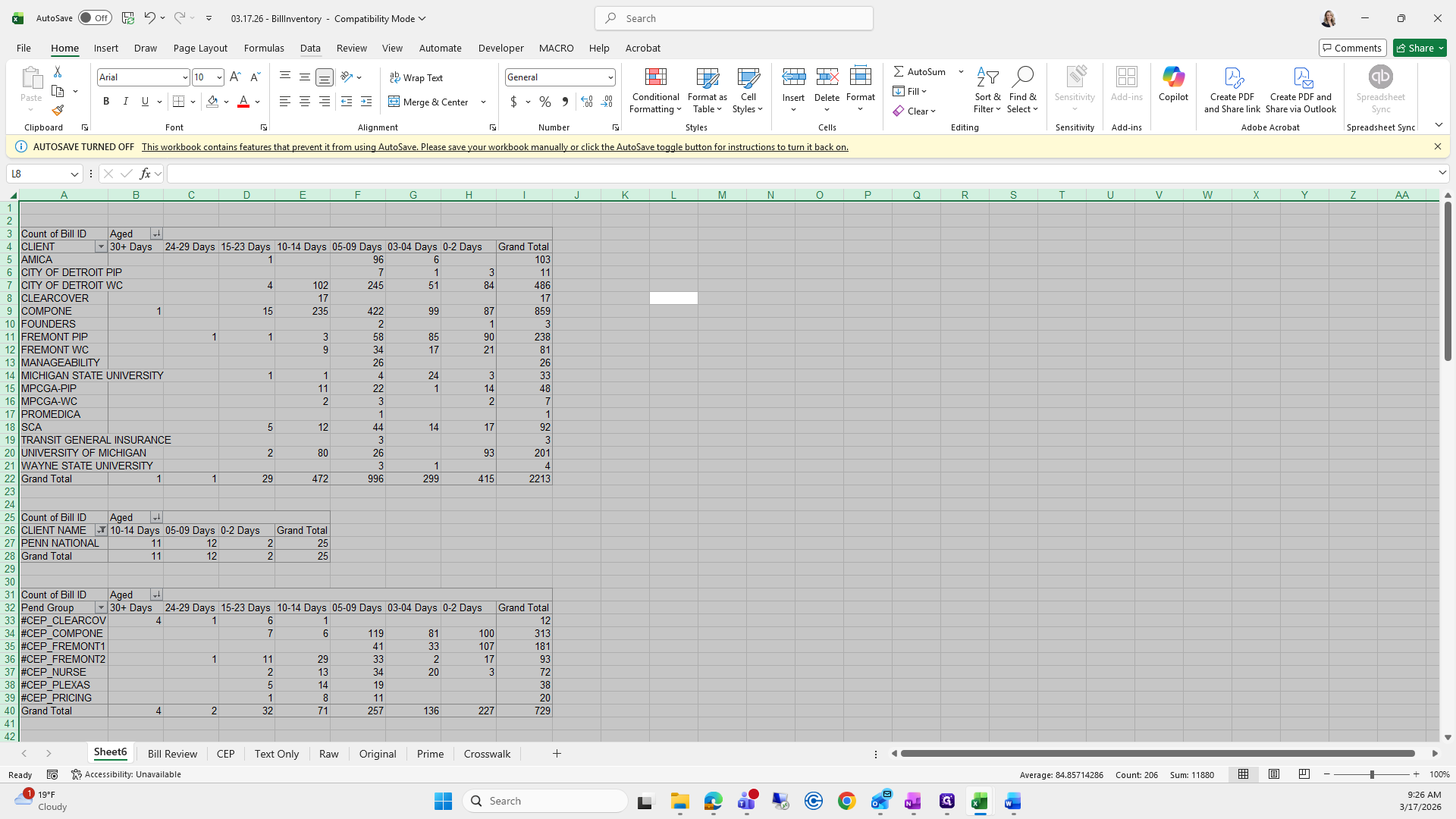
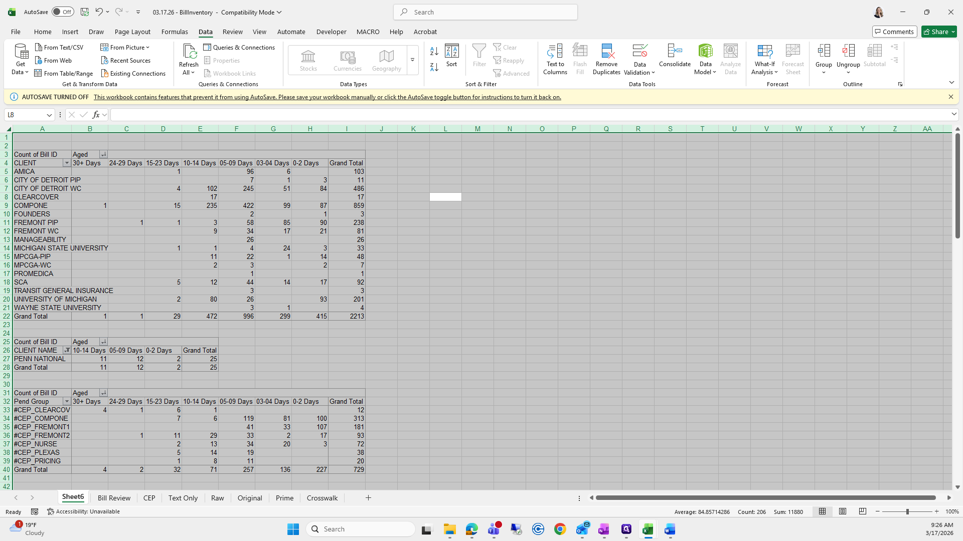
Okay. For the third and final video, we will create pivot tables.
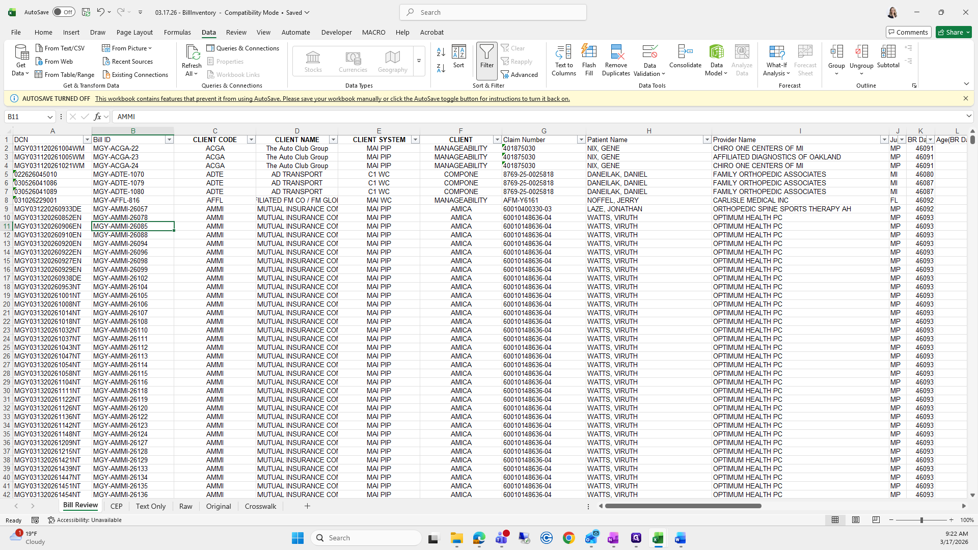
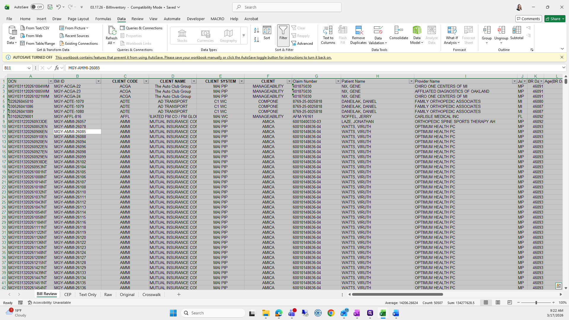
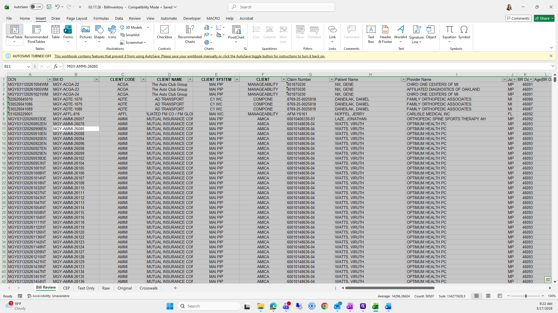
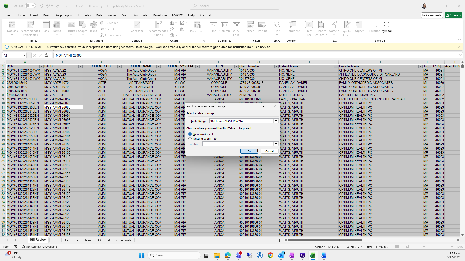
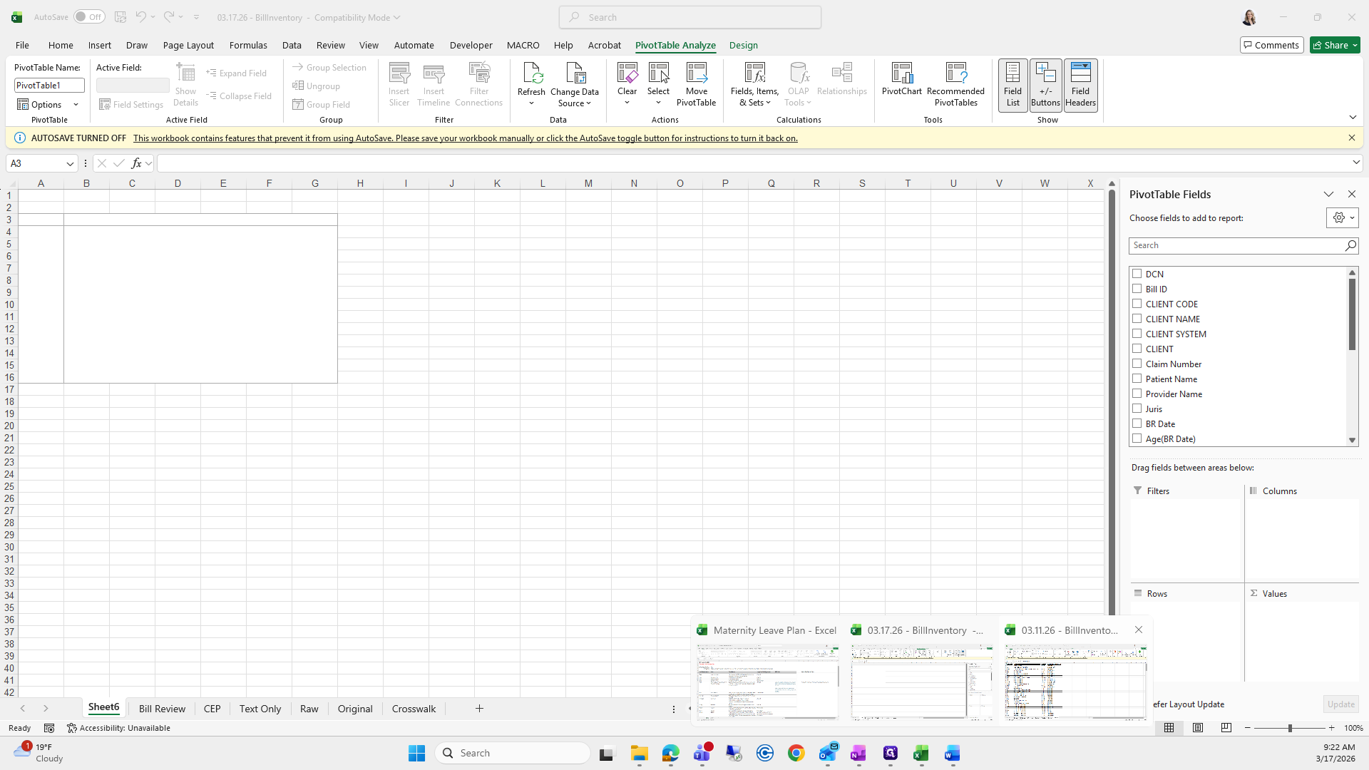
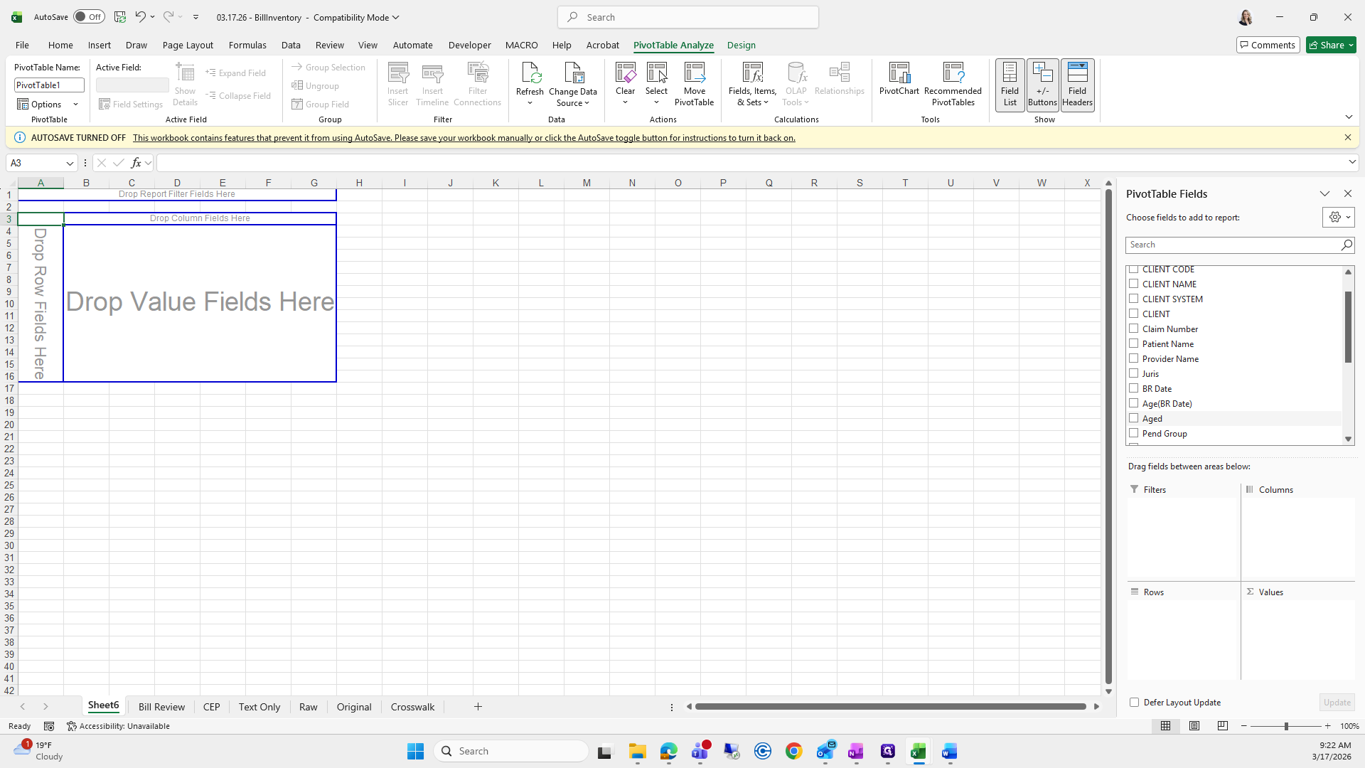
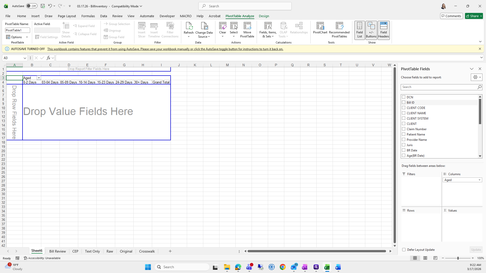
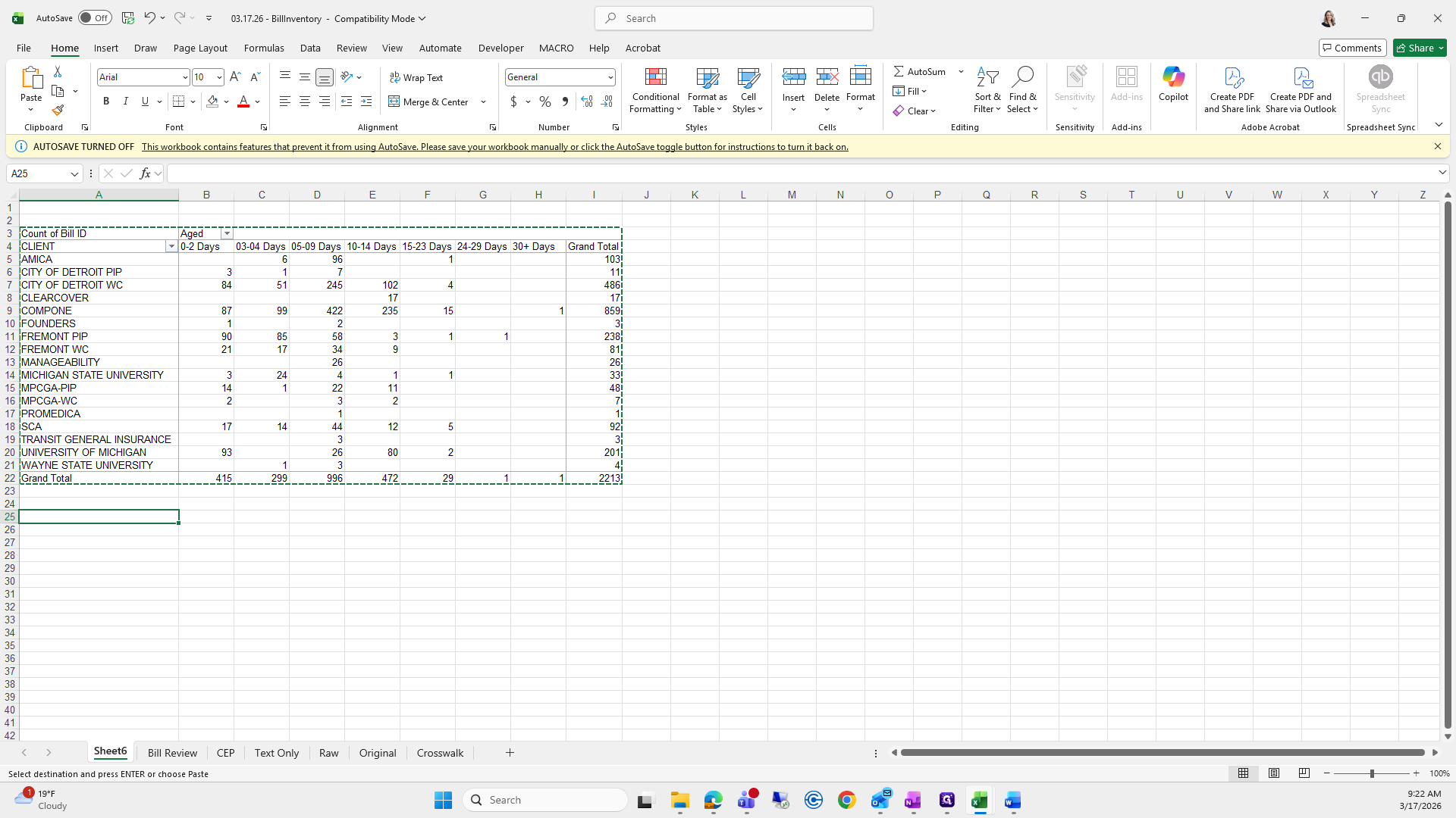
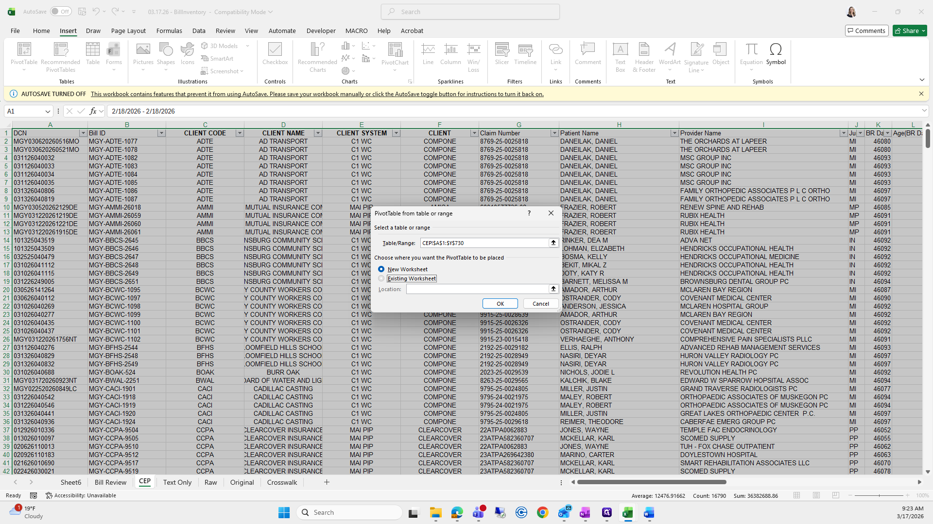
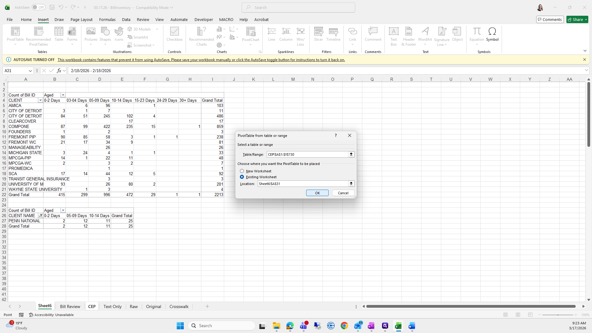
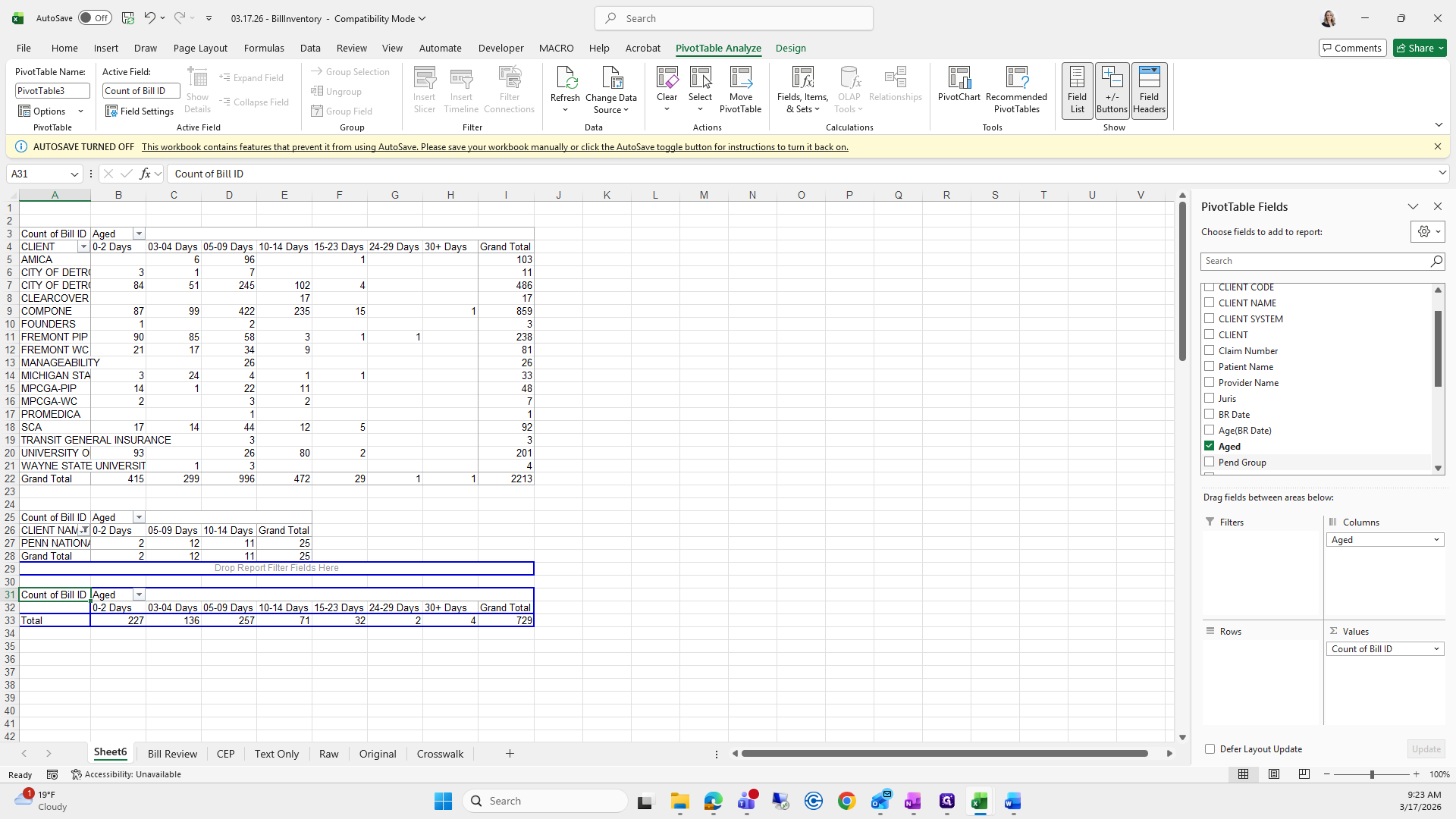
Select All, go to Insert, choose Pivot Table, and click OK. This creates the pivot table for bill review.
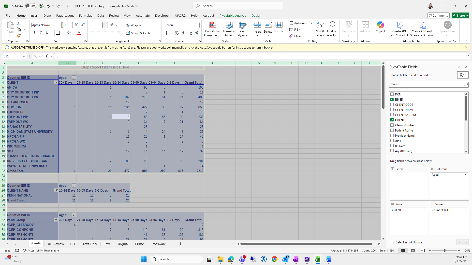
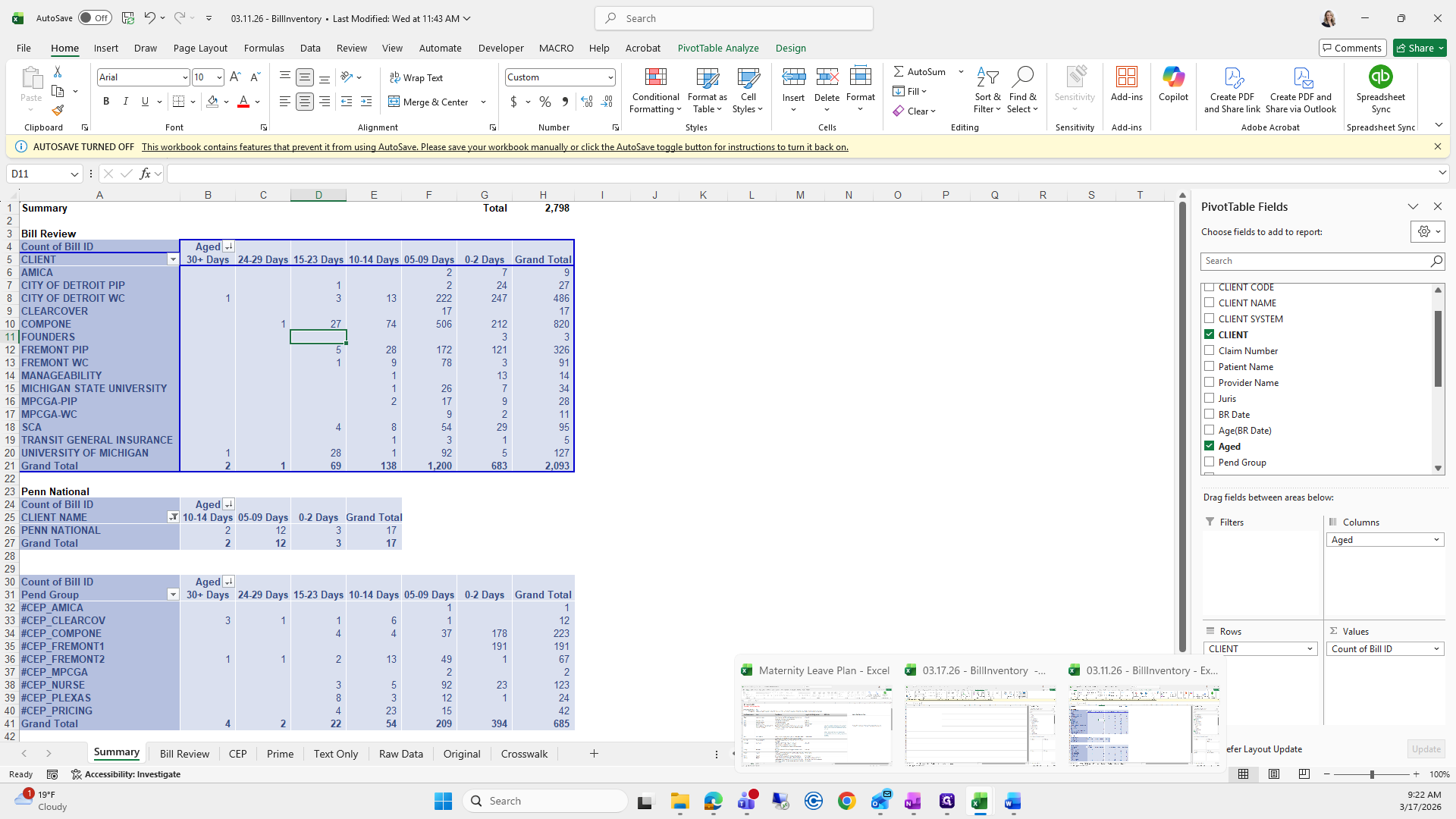
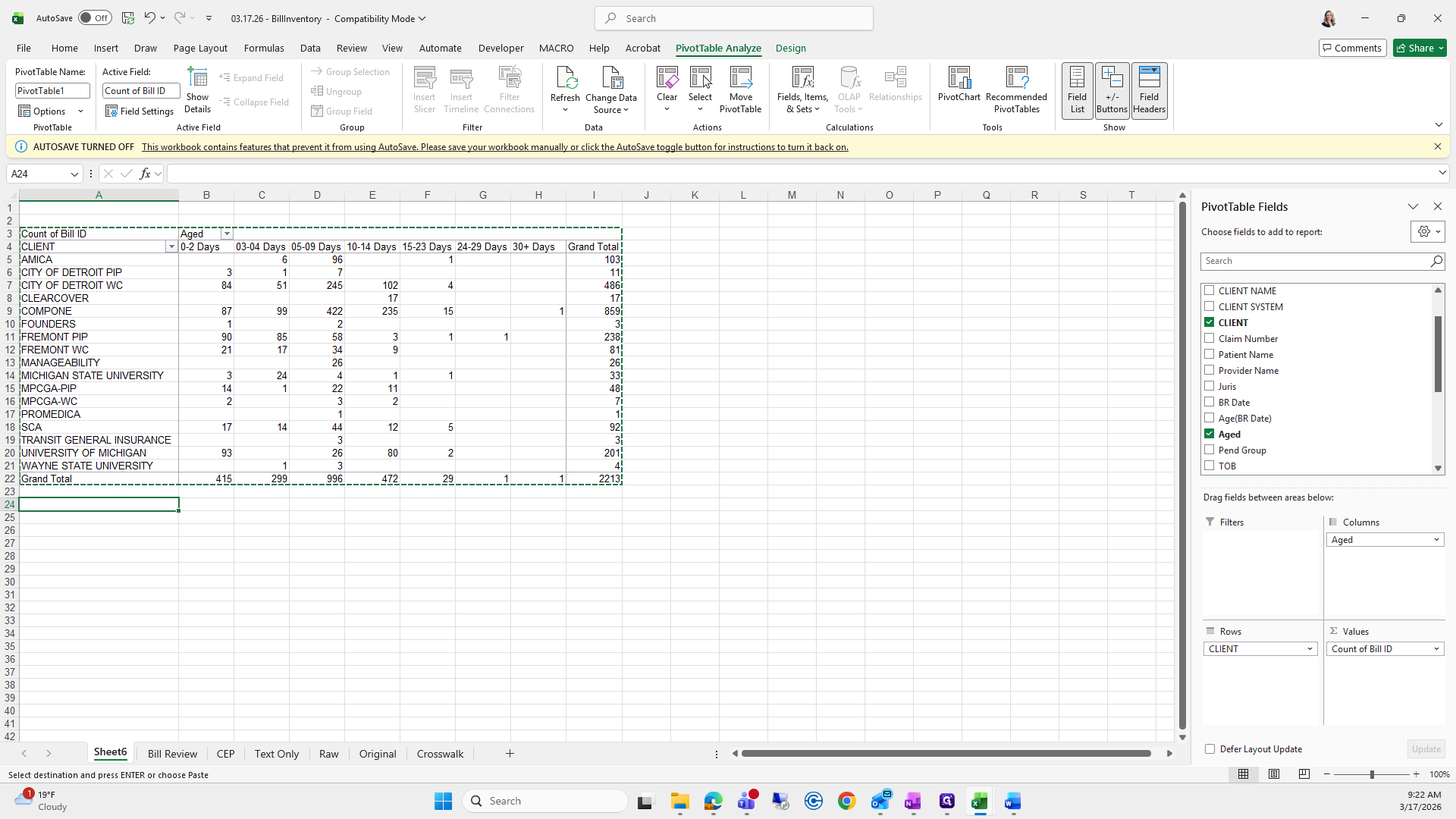
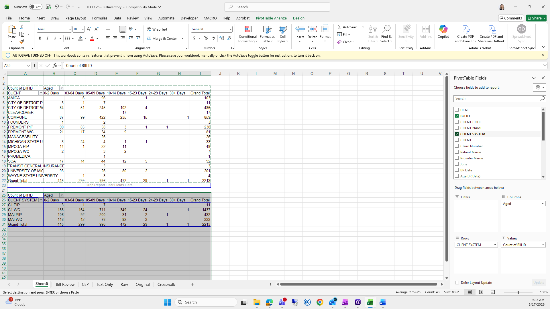
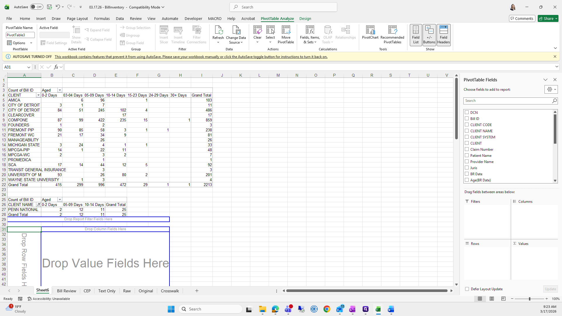
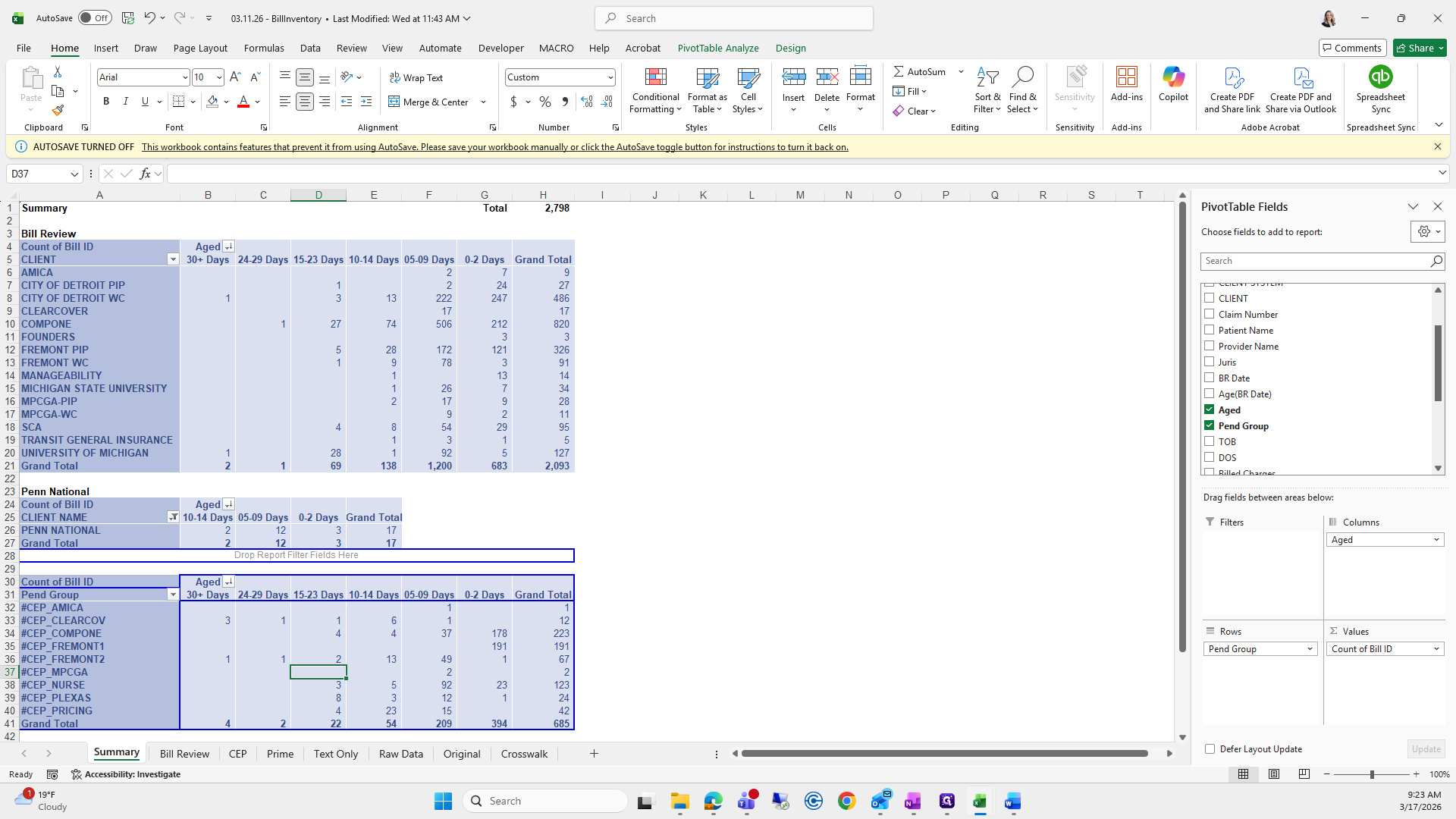
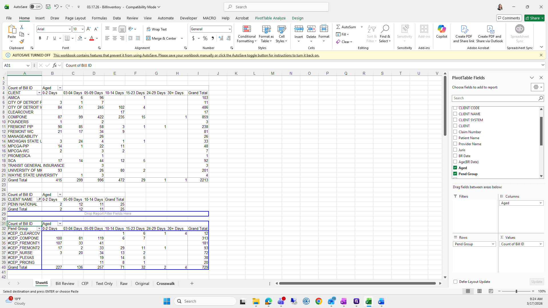
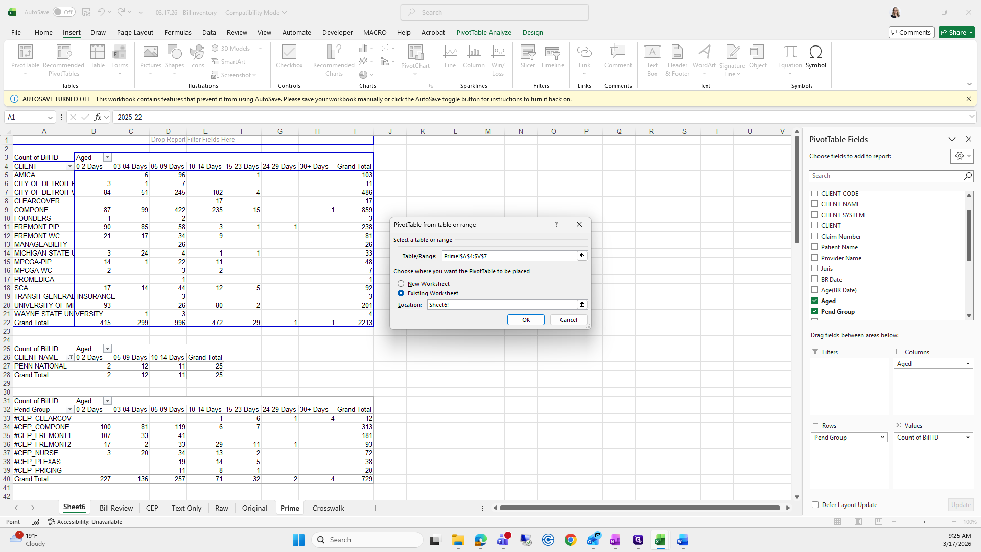
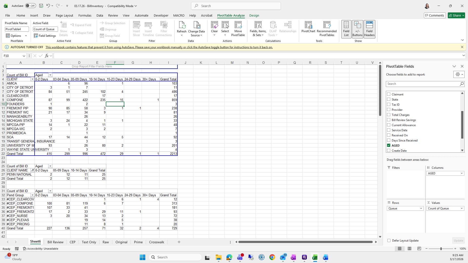
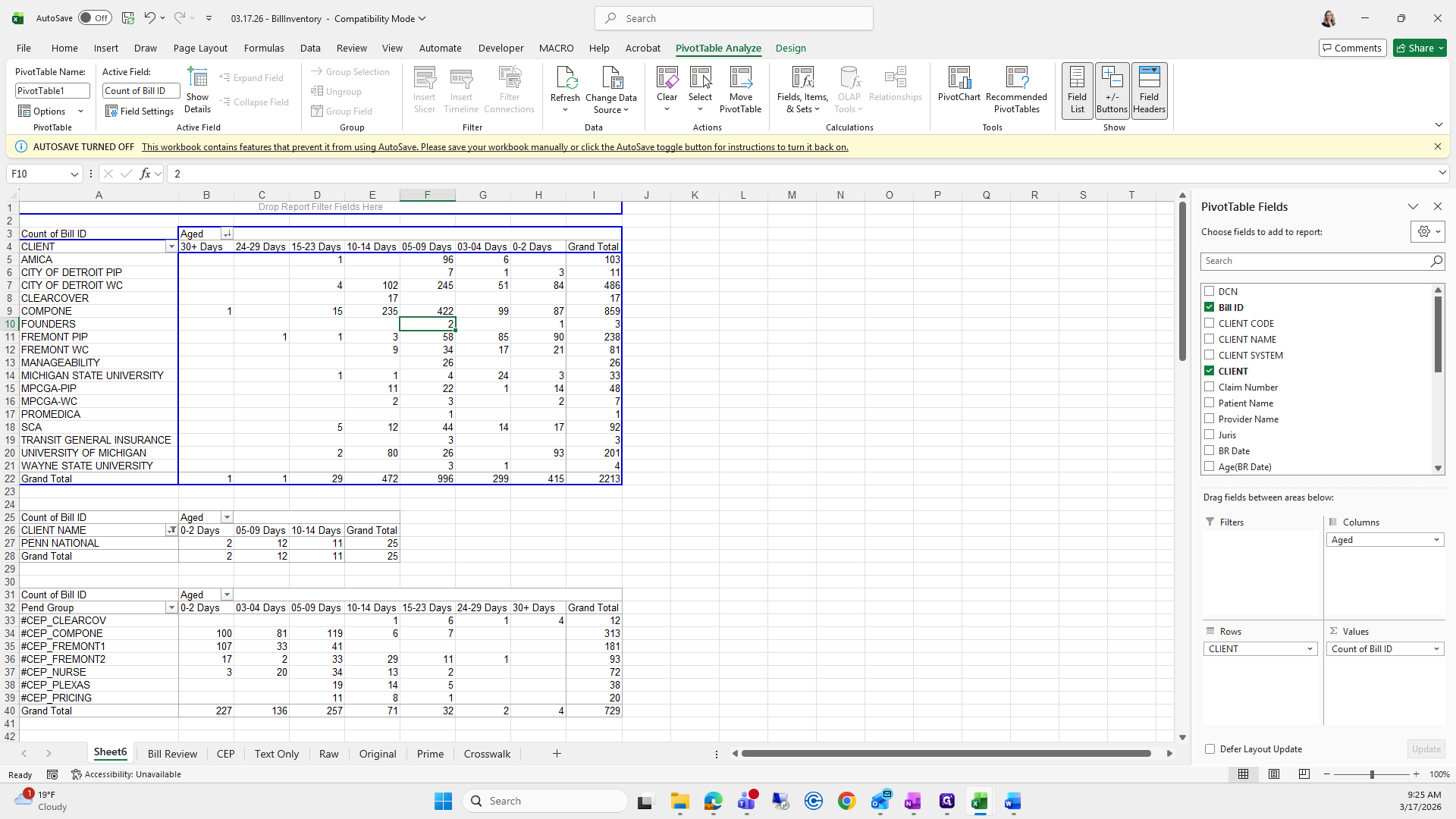
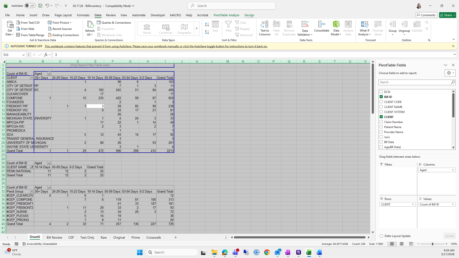
To easily remember which field to choose for columns, rows, and values, I look at previous weeks. I click on the pivot table for bill review, and the fields are Bill ID, Client, and Aged.
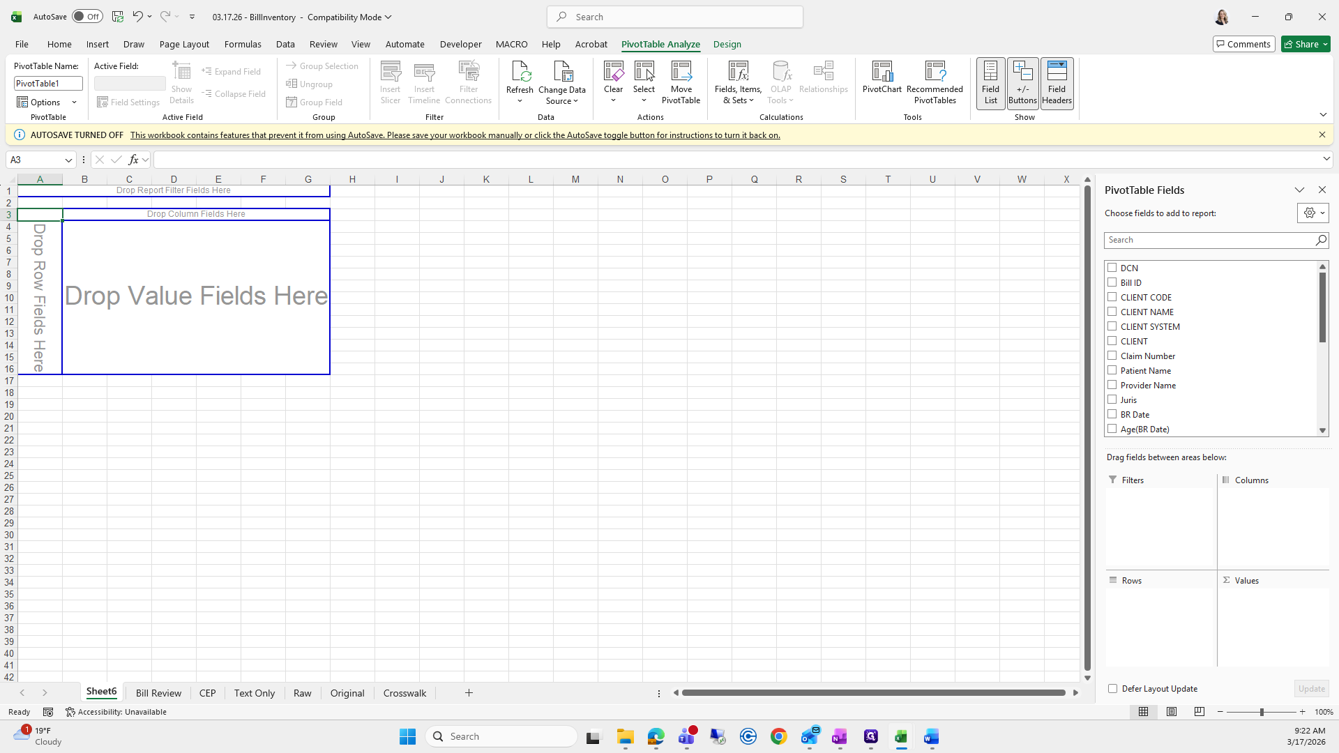
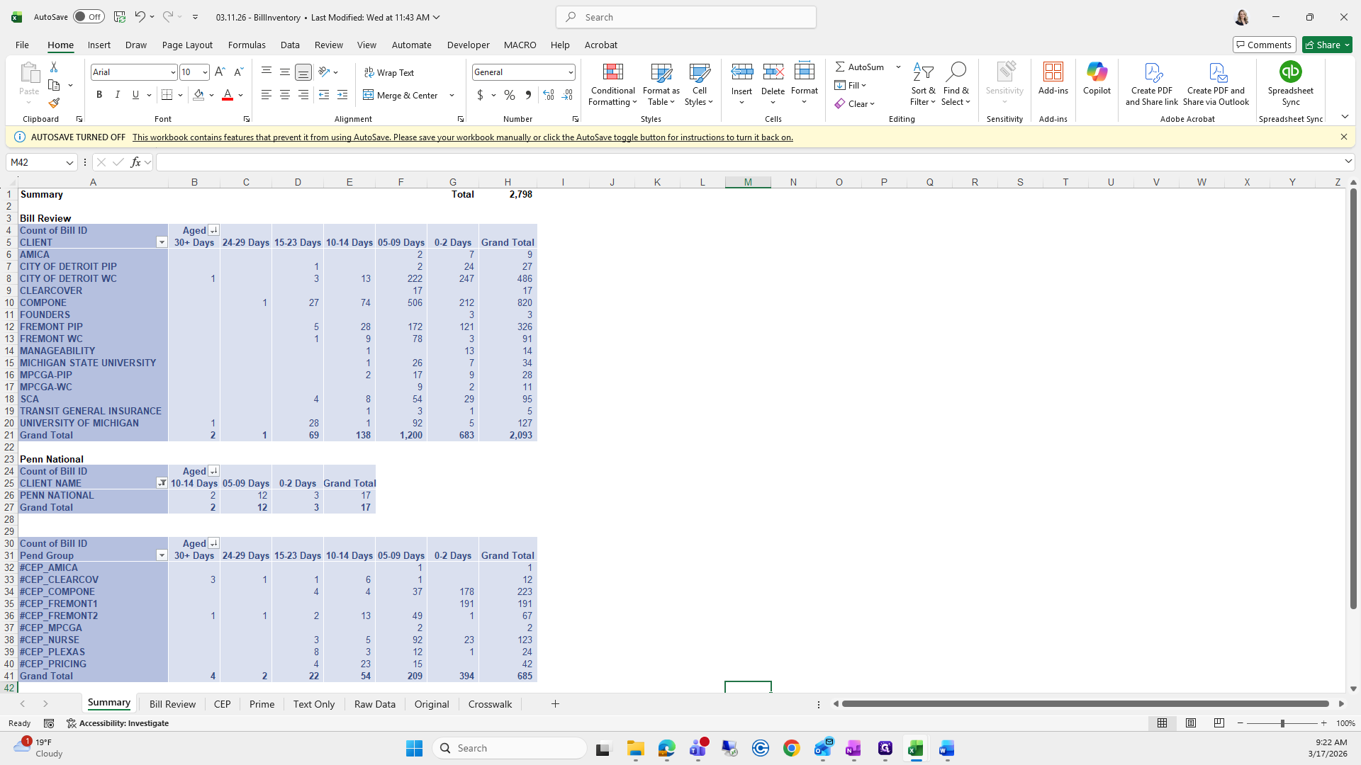
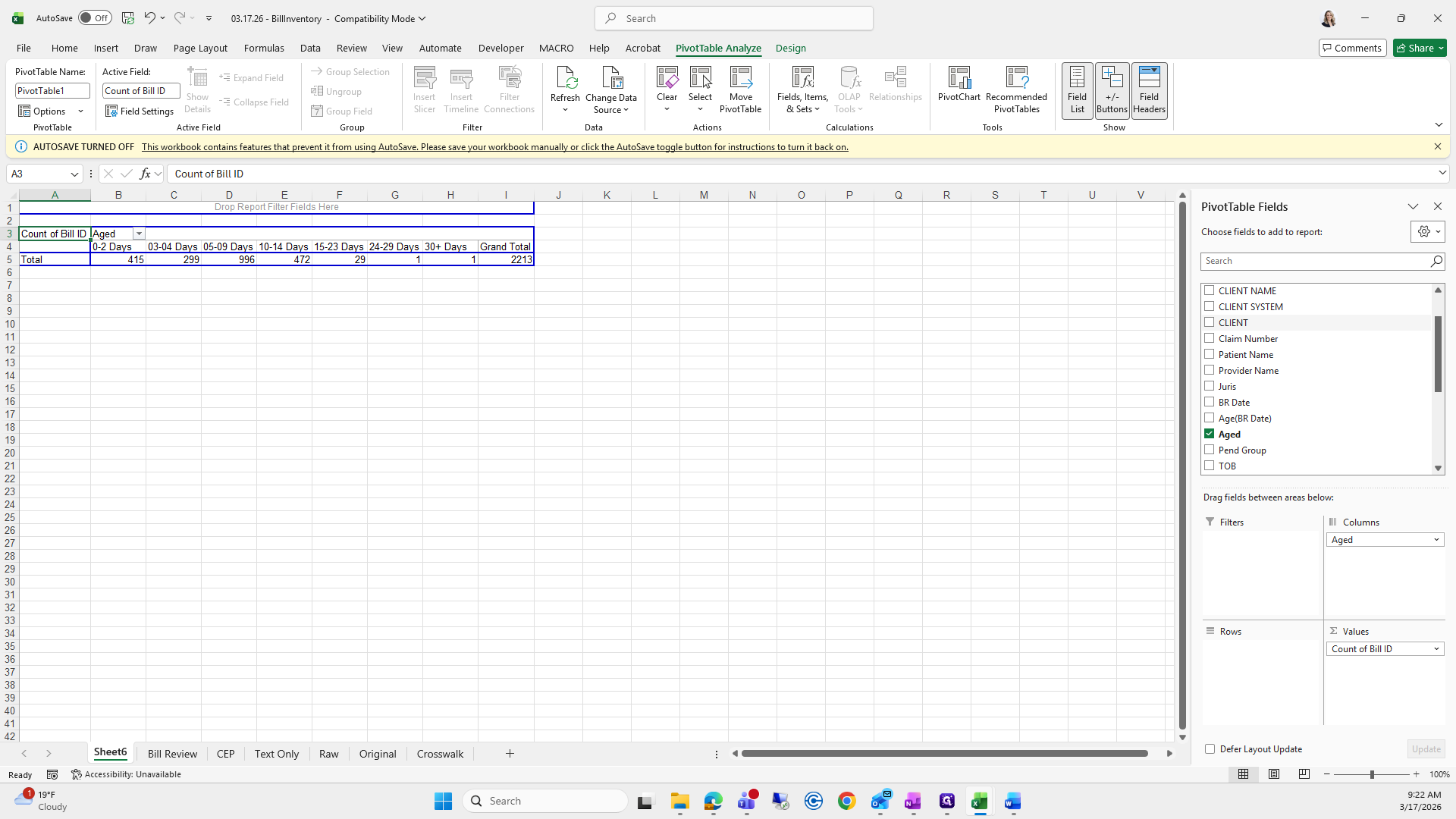
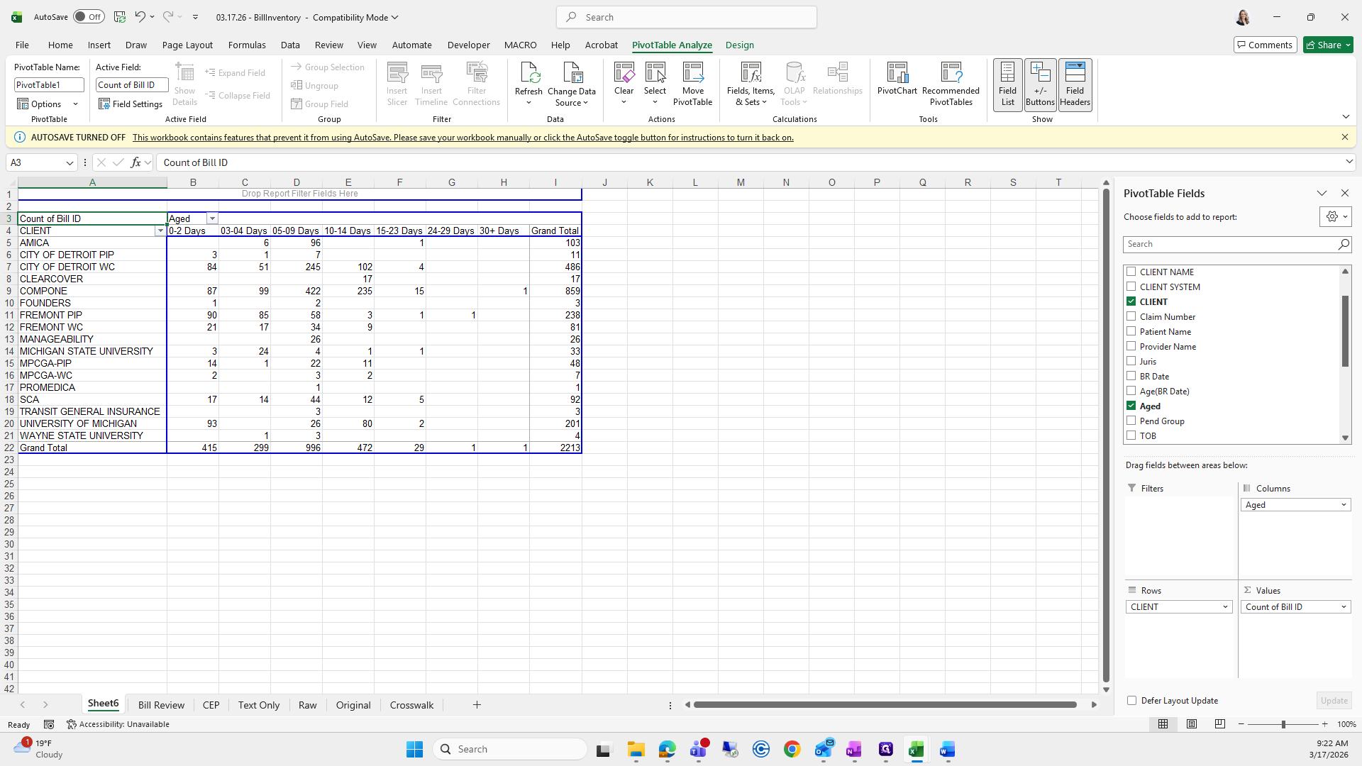
You can see that Bill ID is in Values, Aged is in Columns, and Client is in Rows.
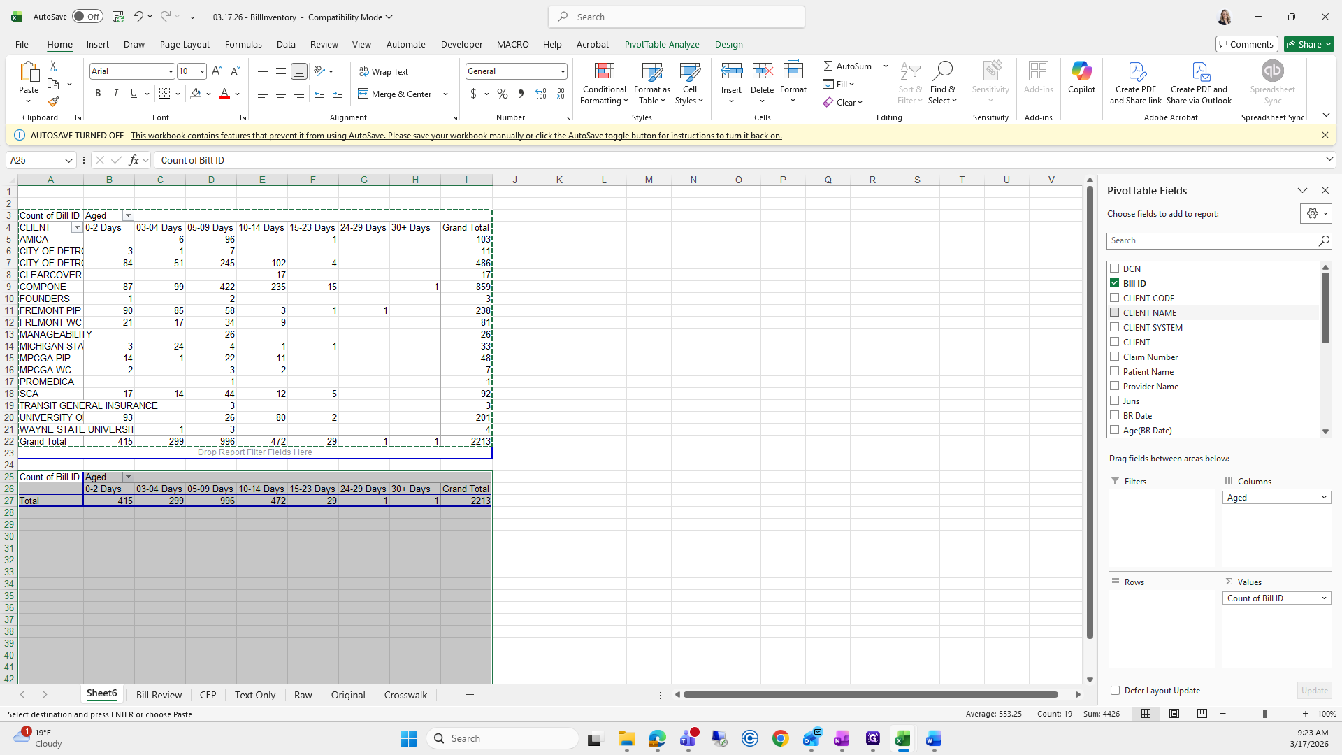
I'll probably forget once I come over here.
Aged is in Columns, Bill ID is in Values, and I forgot what the other one was.
Client is in Rows.
I do that, right? Yes.
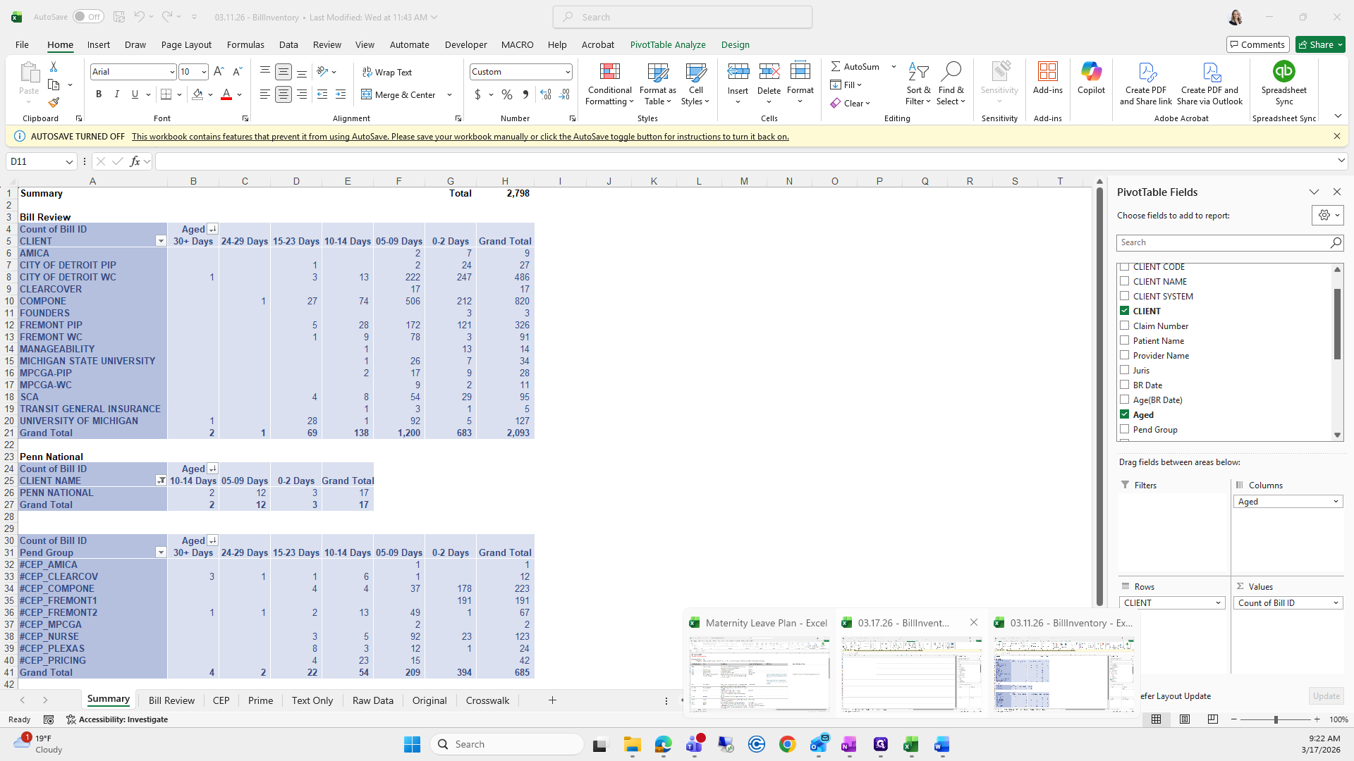
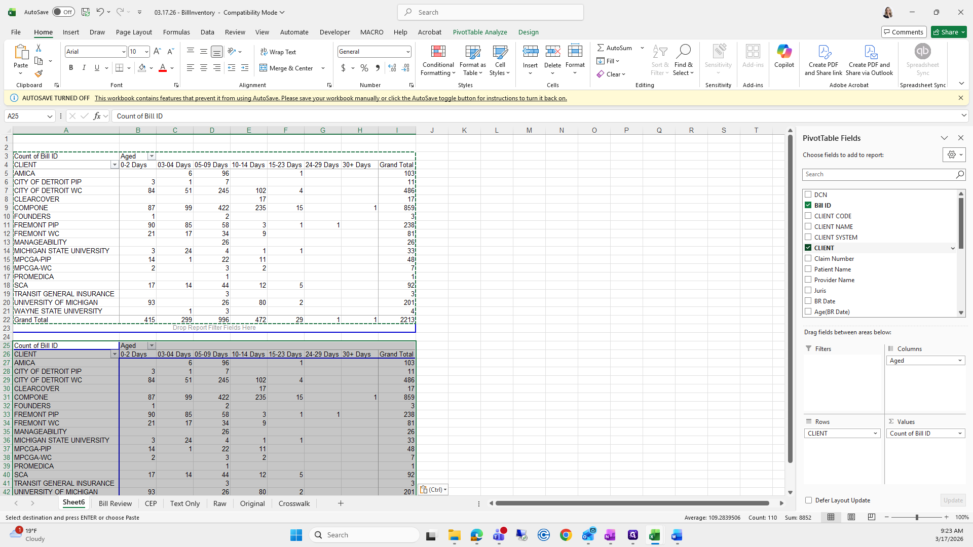
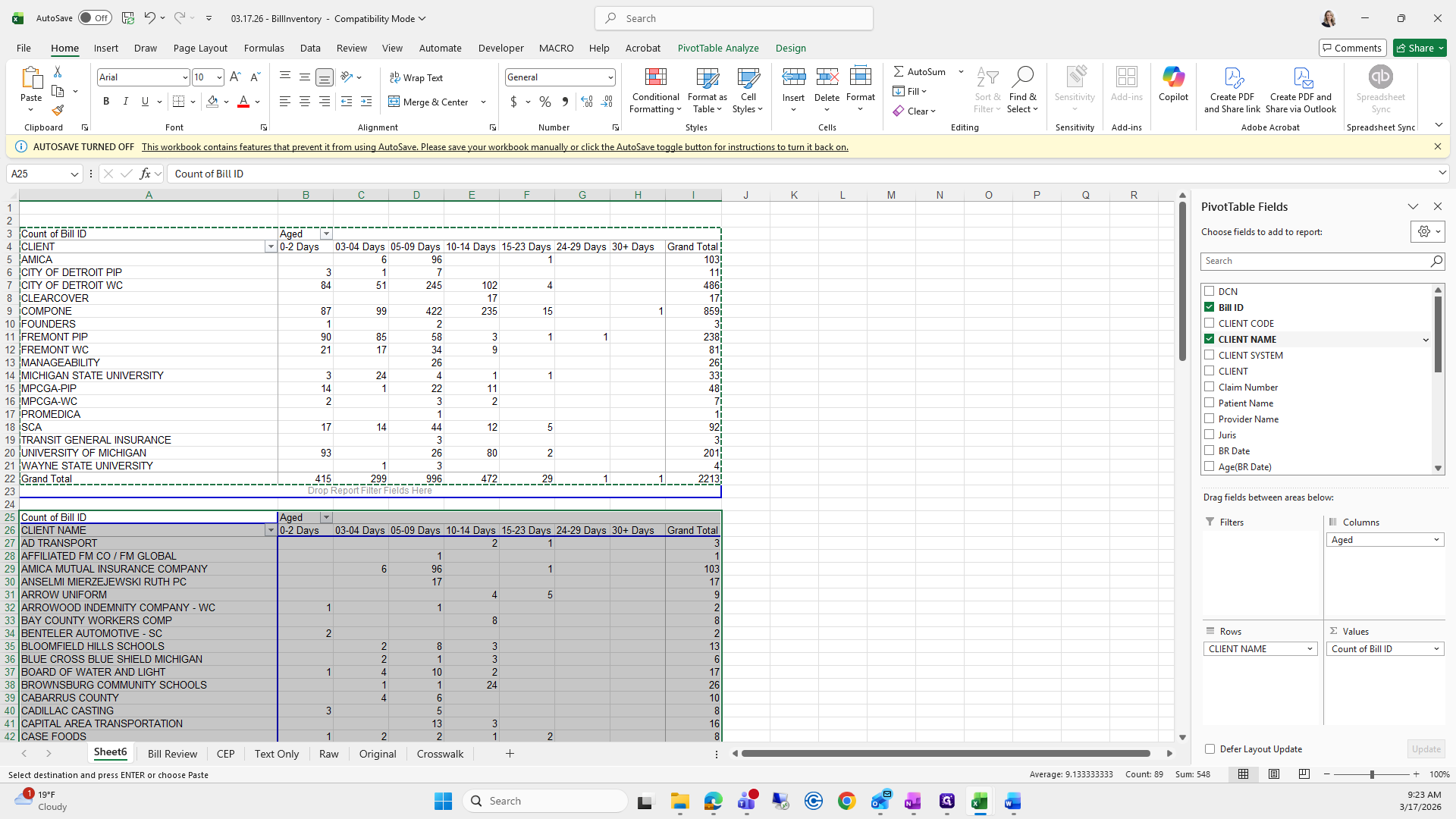
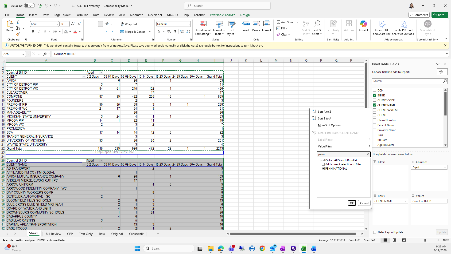
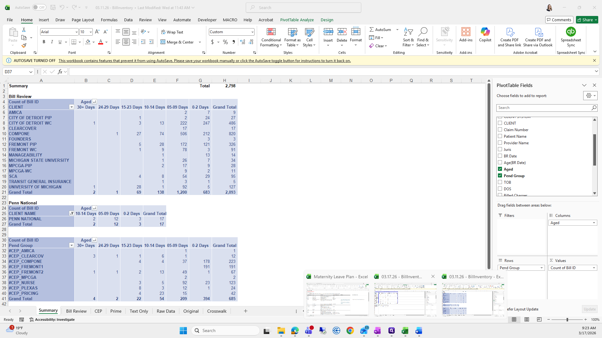
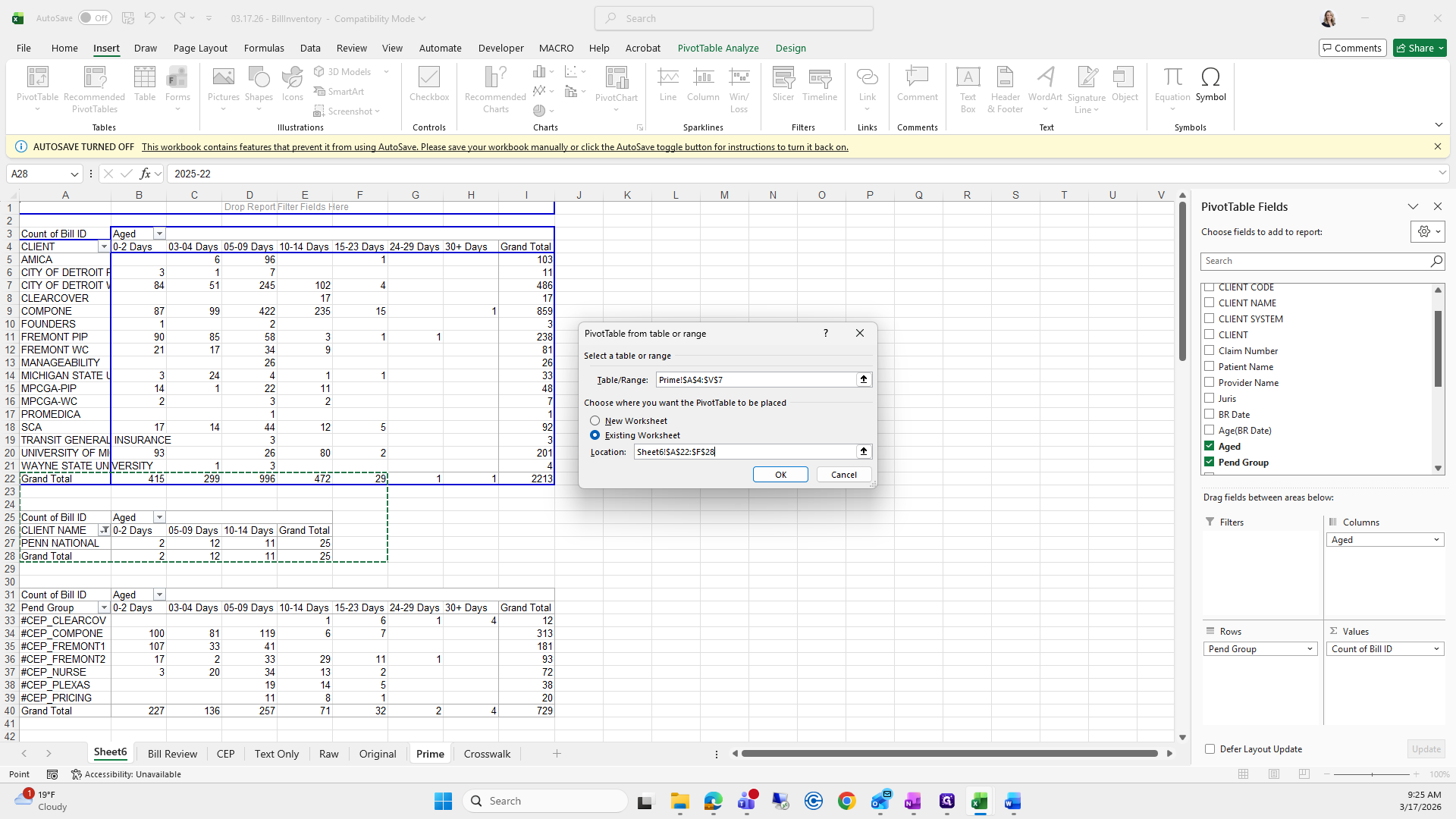
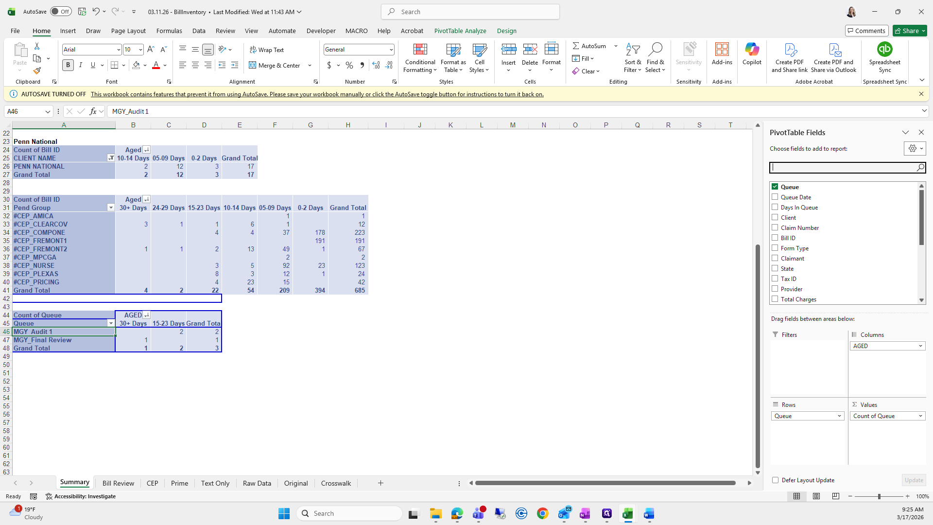
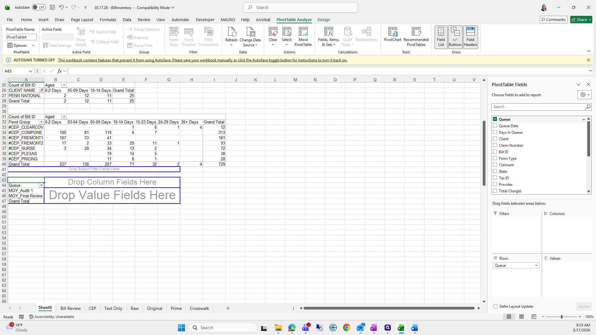
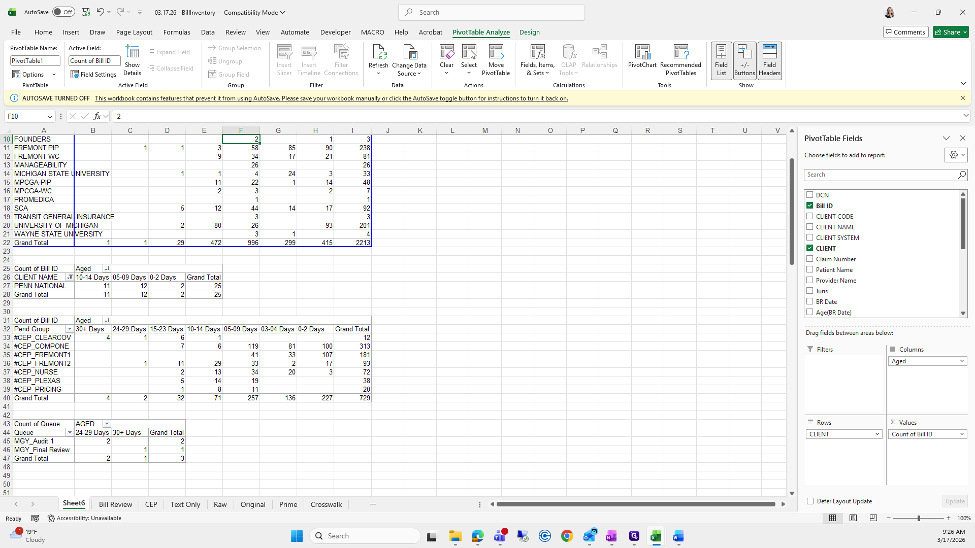
I usually copy and paste this one below because we also need to capture just Pen National.
For this step, since I copied and pasted, I'll remove "Client" and use "Client Name." Then, I'll filter the client name to just "Pen National" and click "Okay."
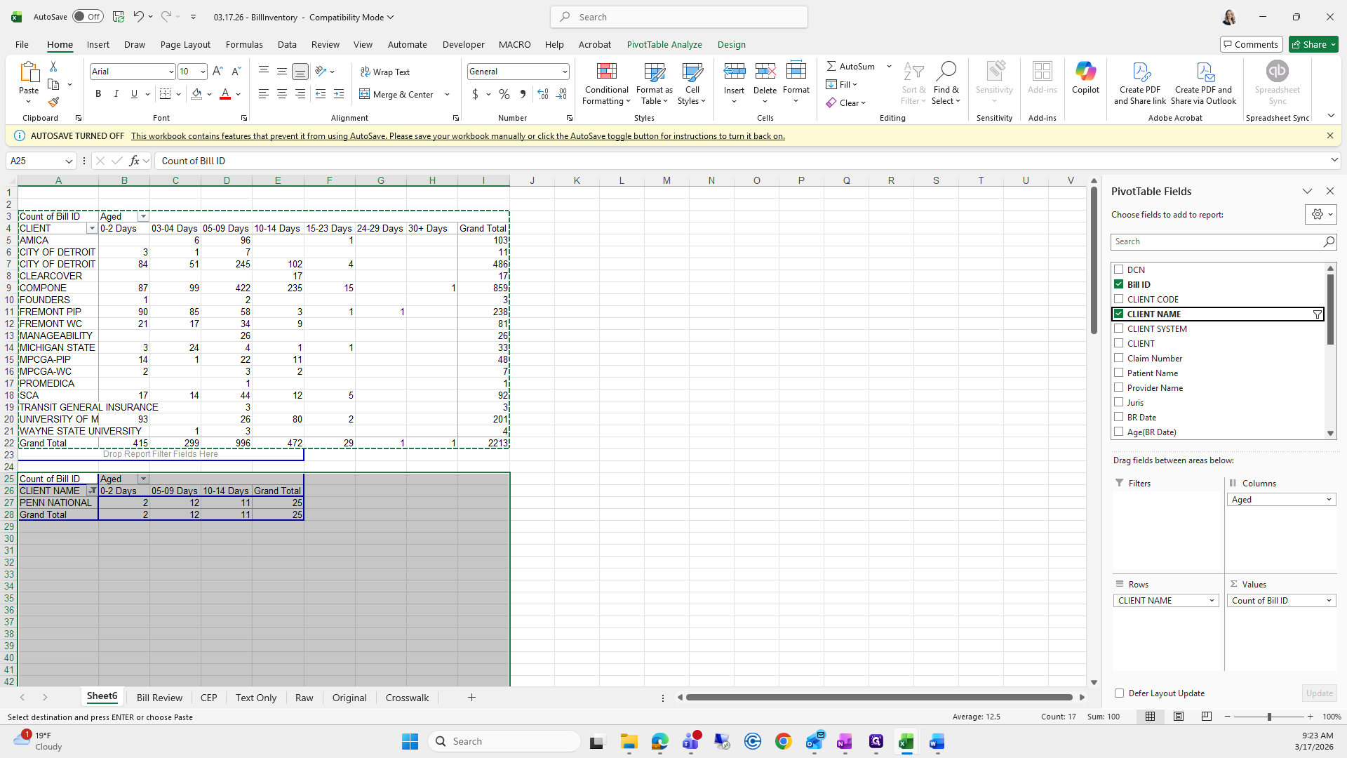
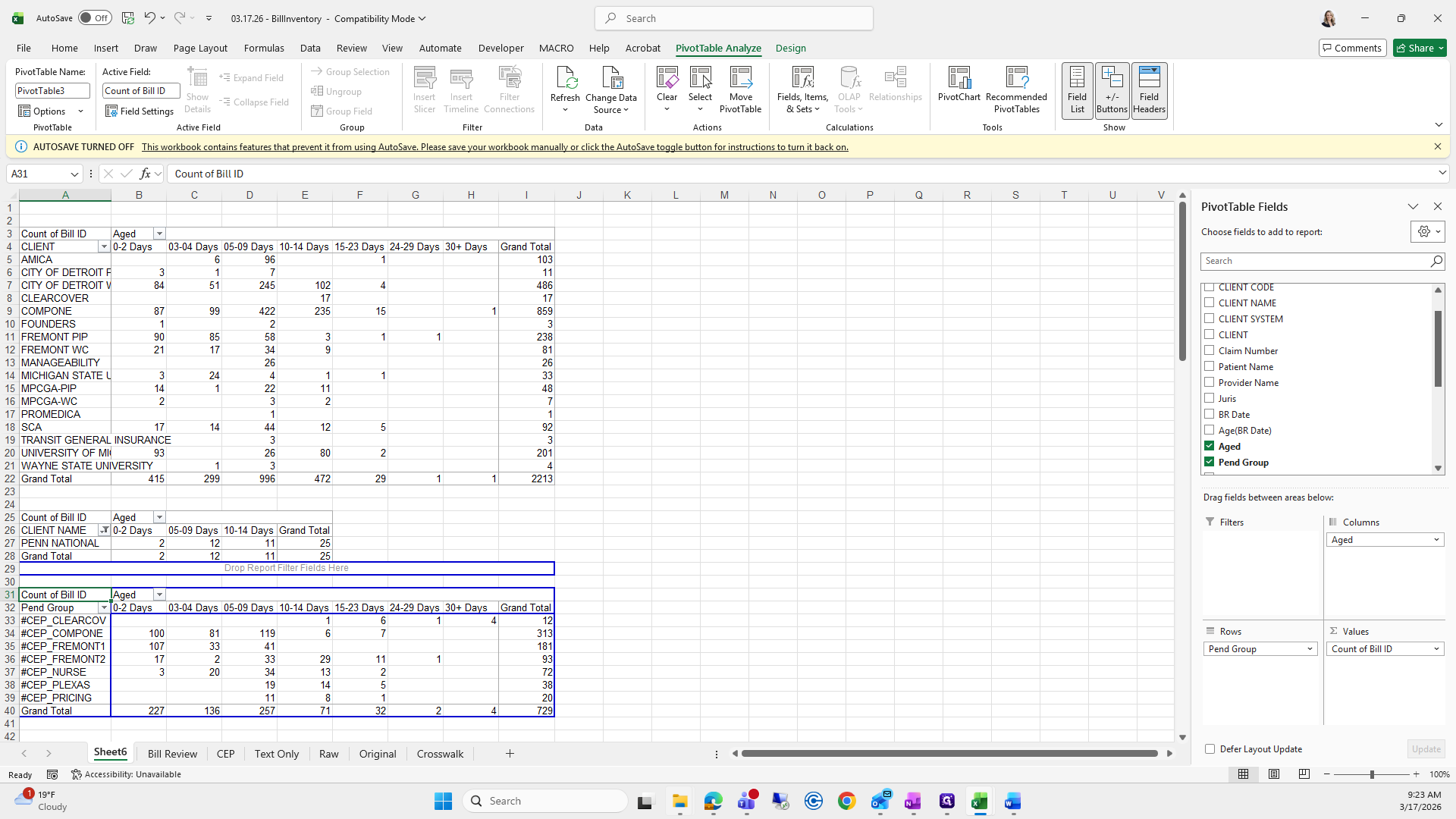
That looks good. Next, we'll do it for CEP.
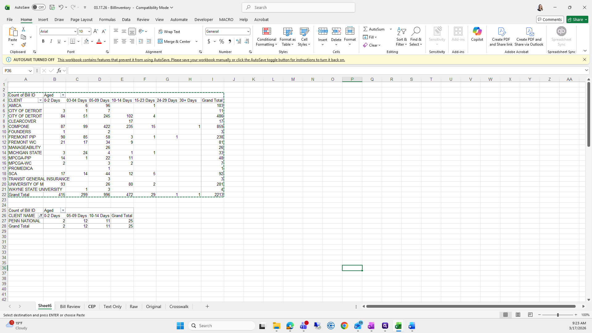
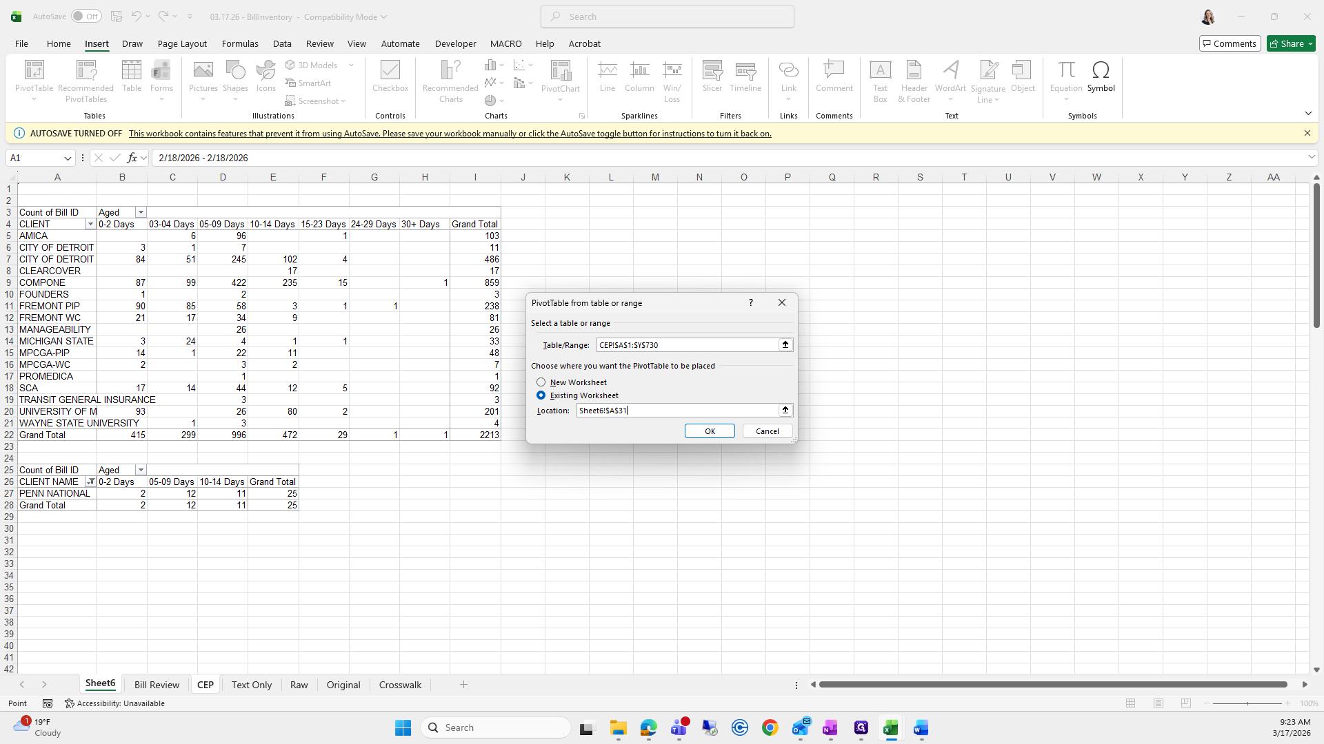
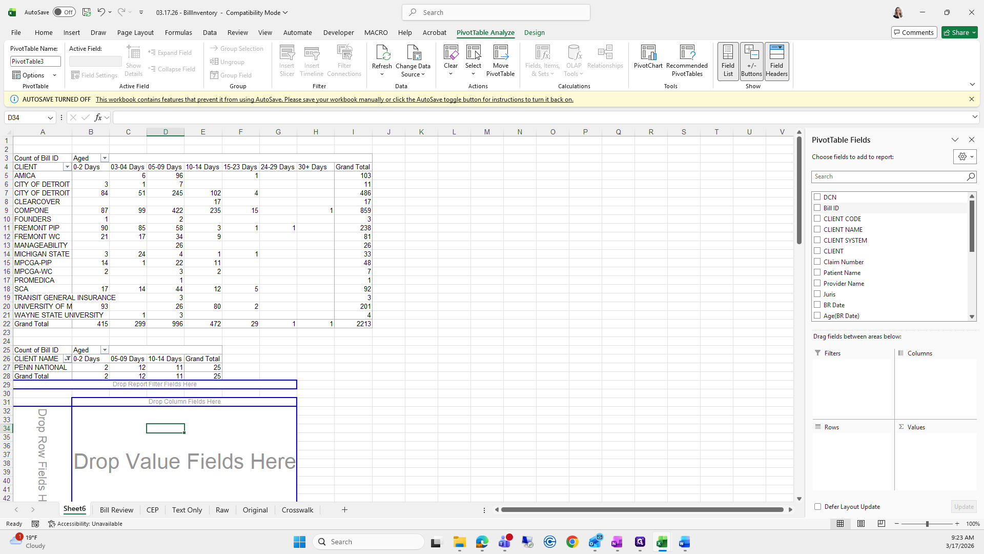
Select All, Insert, Pivot Table, Existing Worksheet.
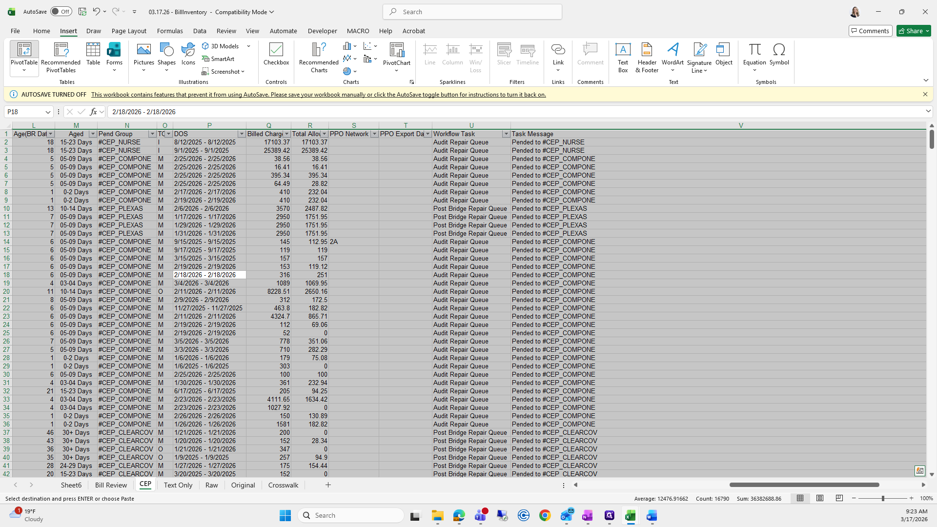

We will go underneath and click OK.
Again, I will go back to the previous worksheet.
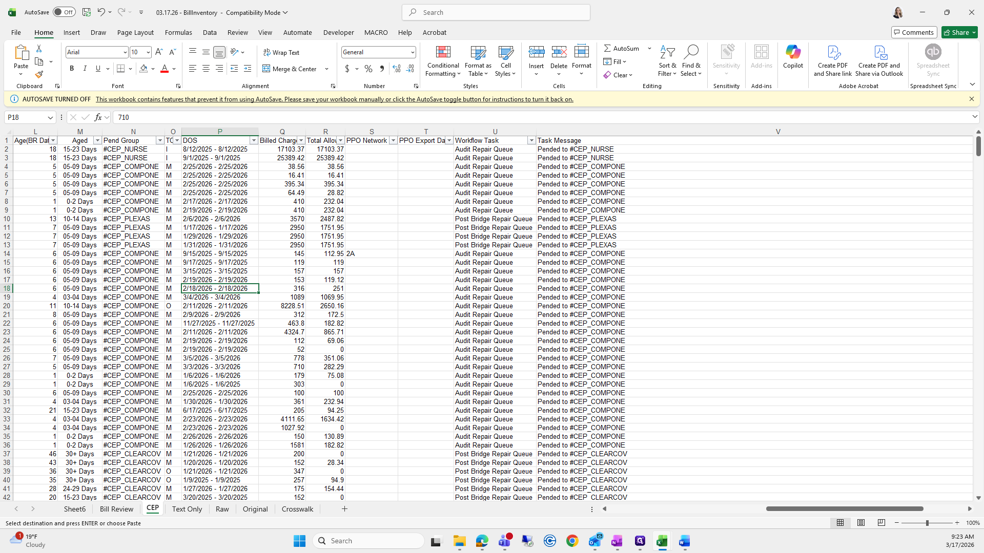
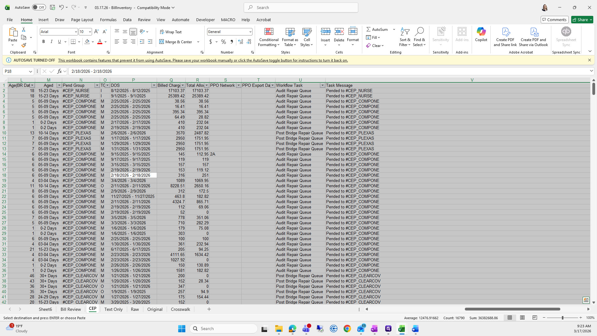
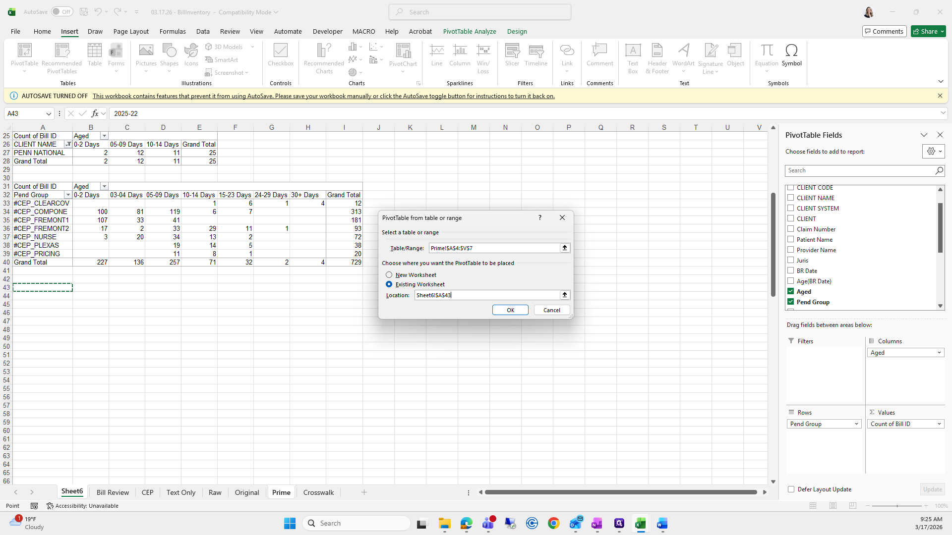
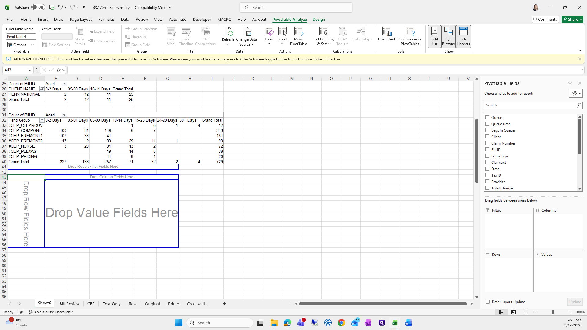
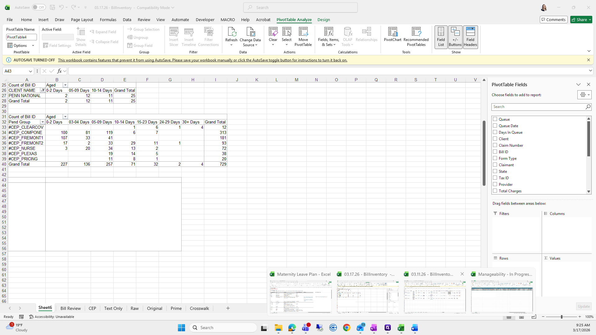
We will go down to this one. For CEP, it's Bill ID, Aged, and Pen Group. Aged Columns, Accountable ID and Values, and Pen Group in Rows. Now we will return to R, select Bill ID, Aged, and Pending Group.

Okay. Now we have one left.
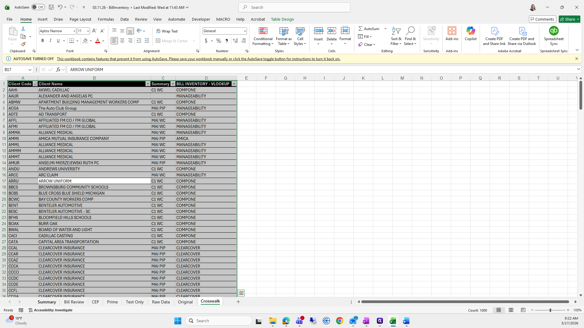
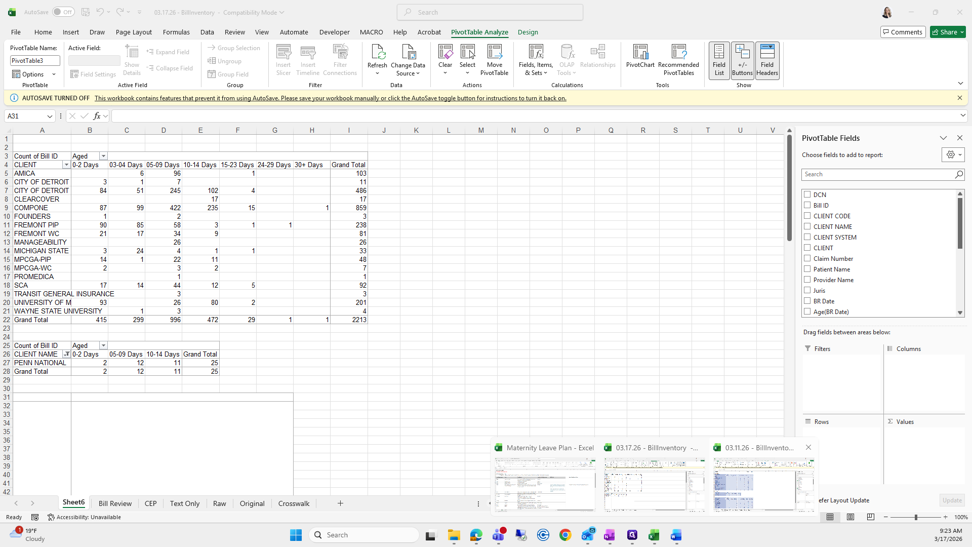
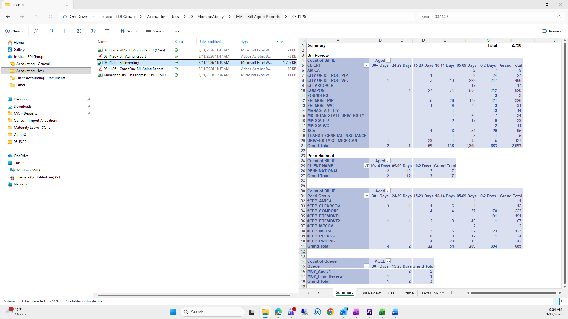
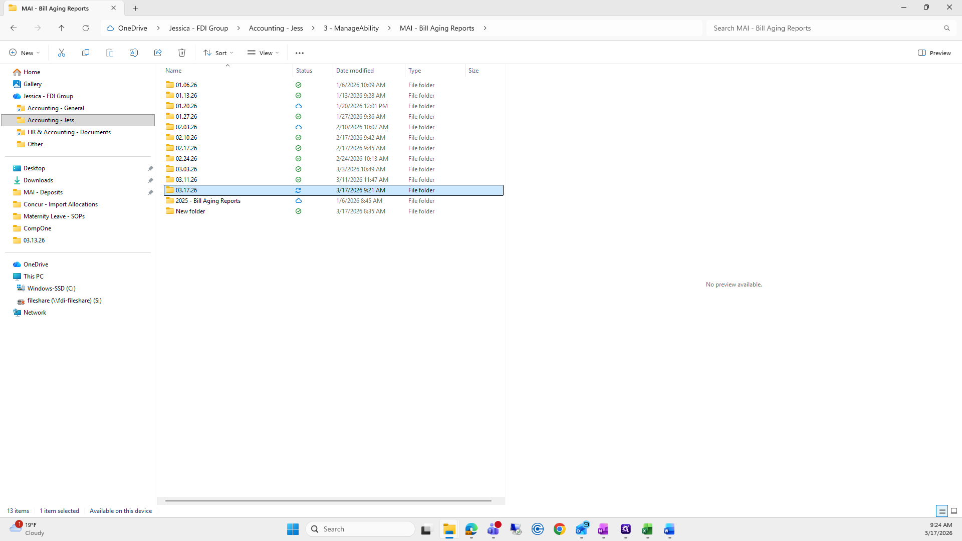
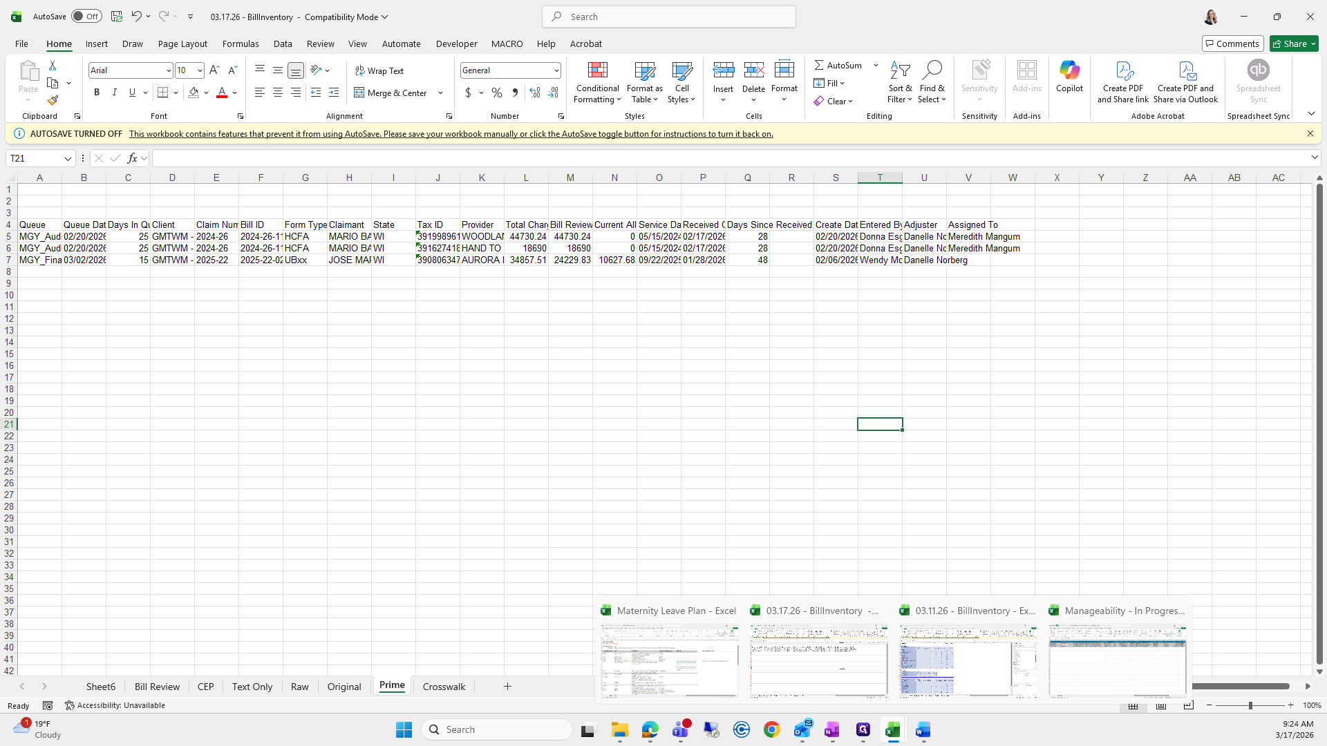
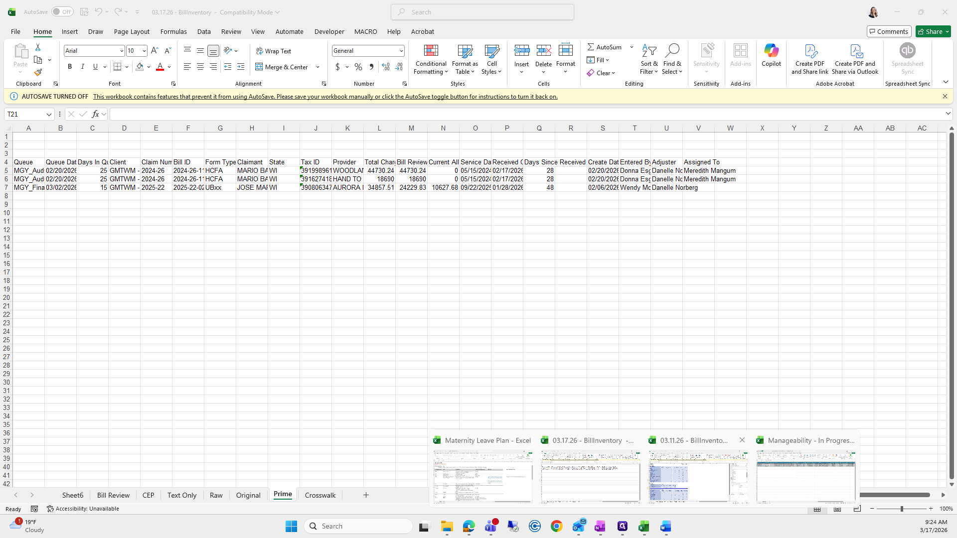
We need to open the file Meredith sent us.
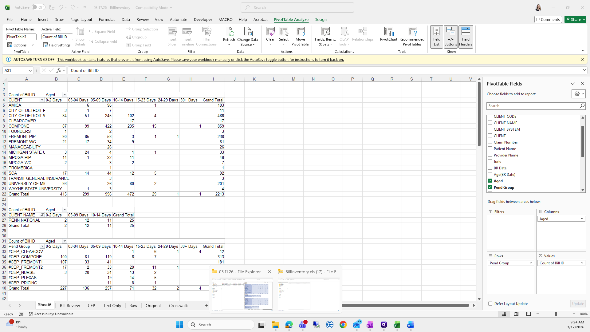
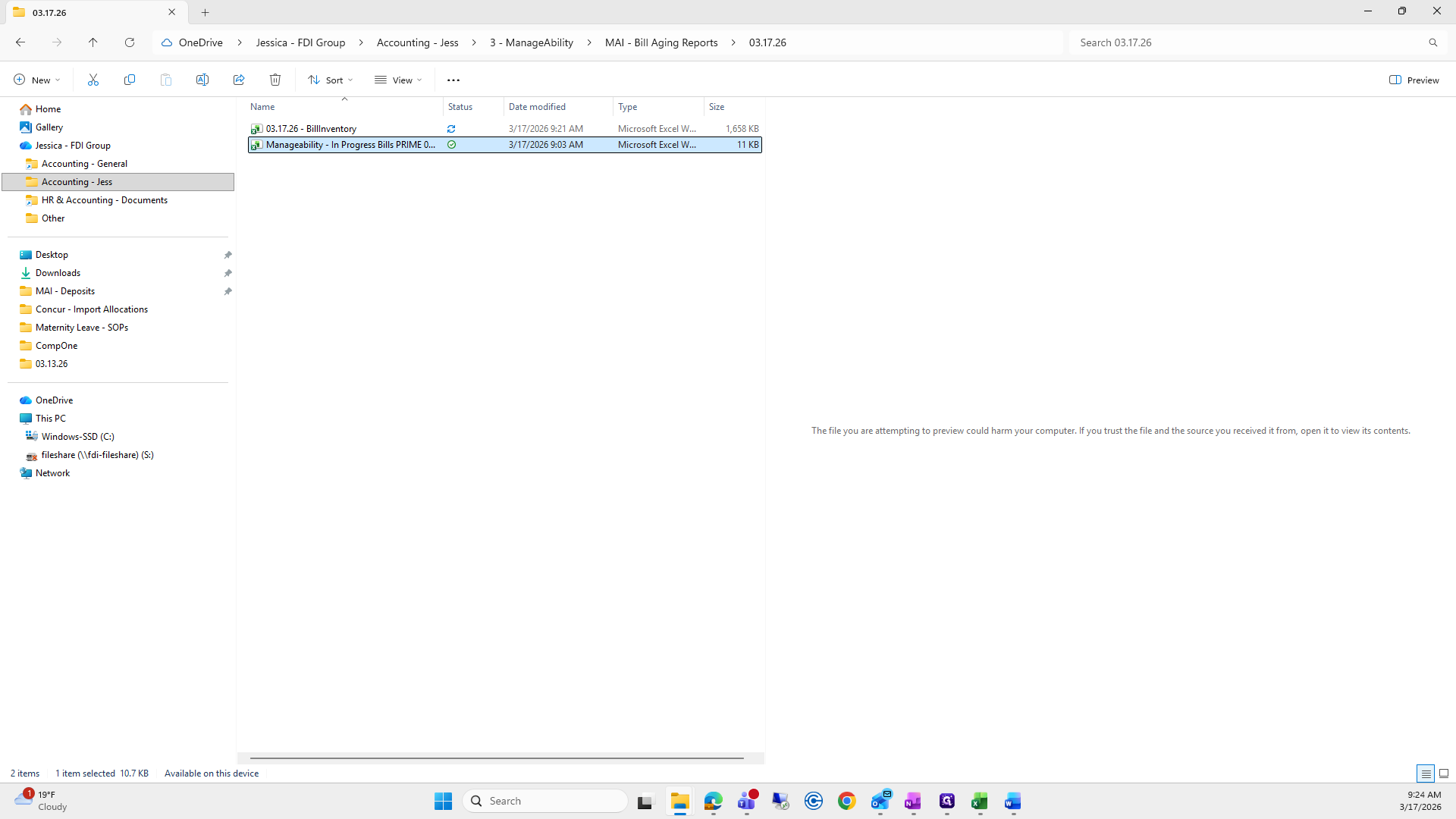
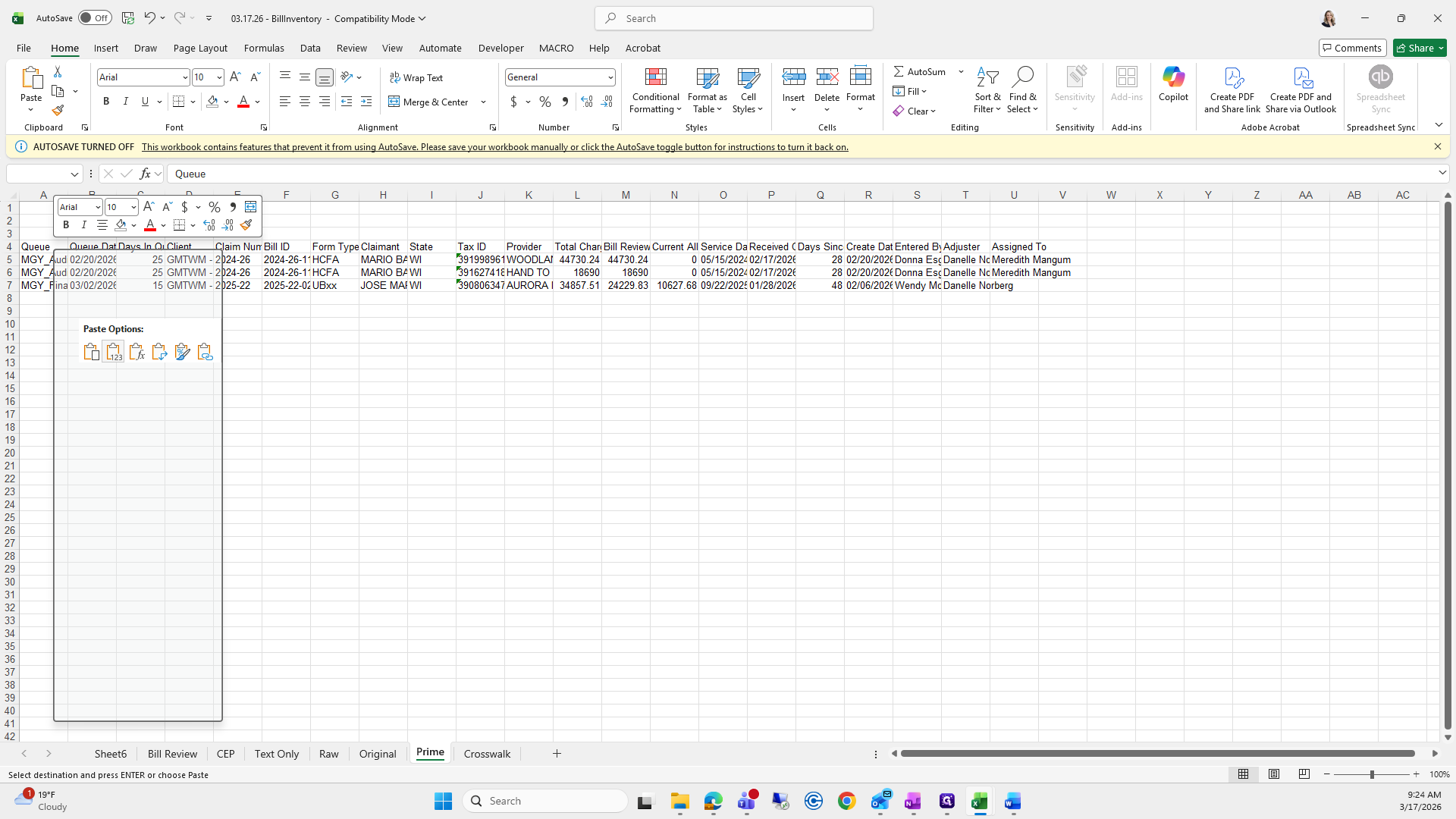
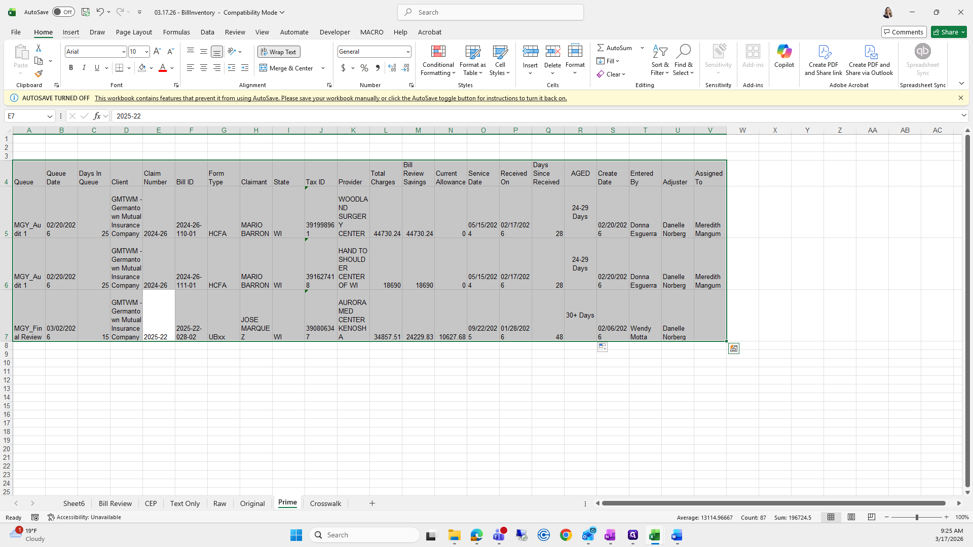
We will select All, then Copy.
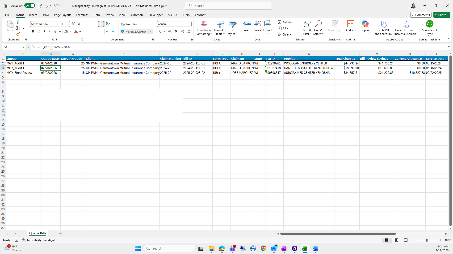
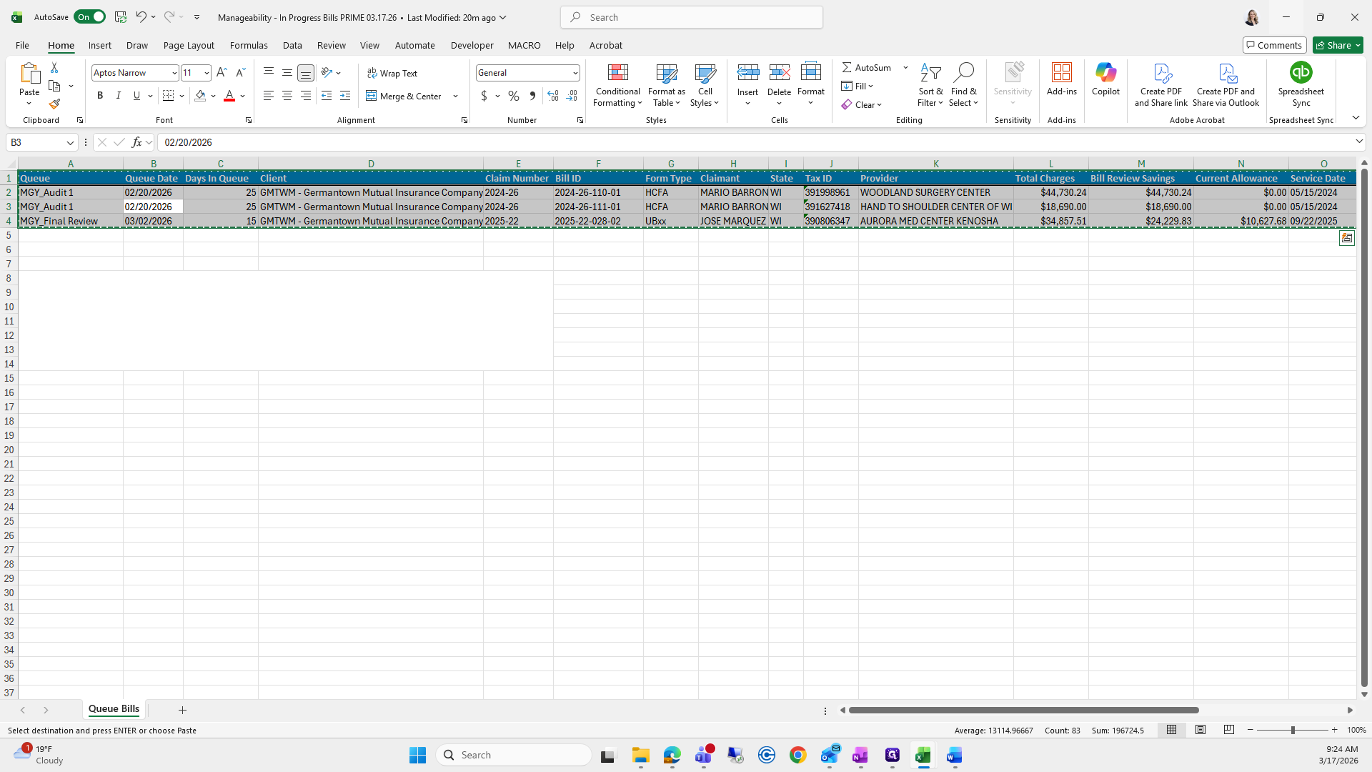
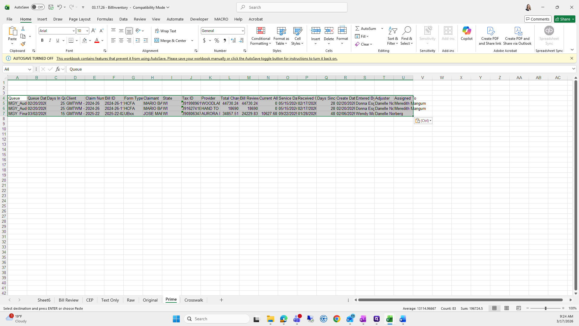
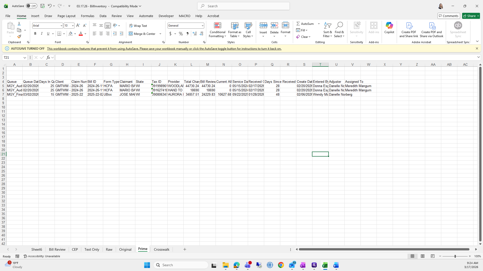
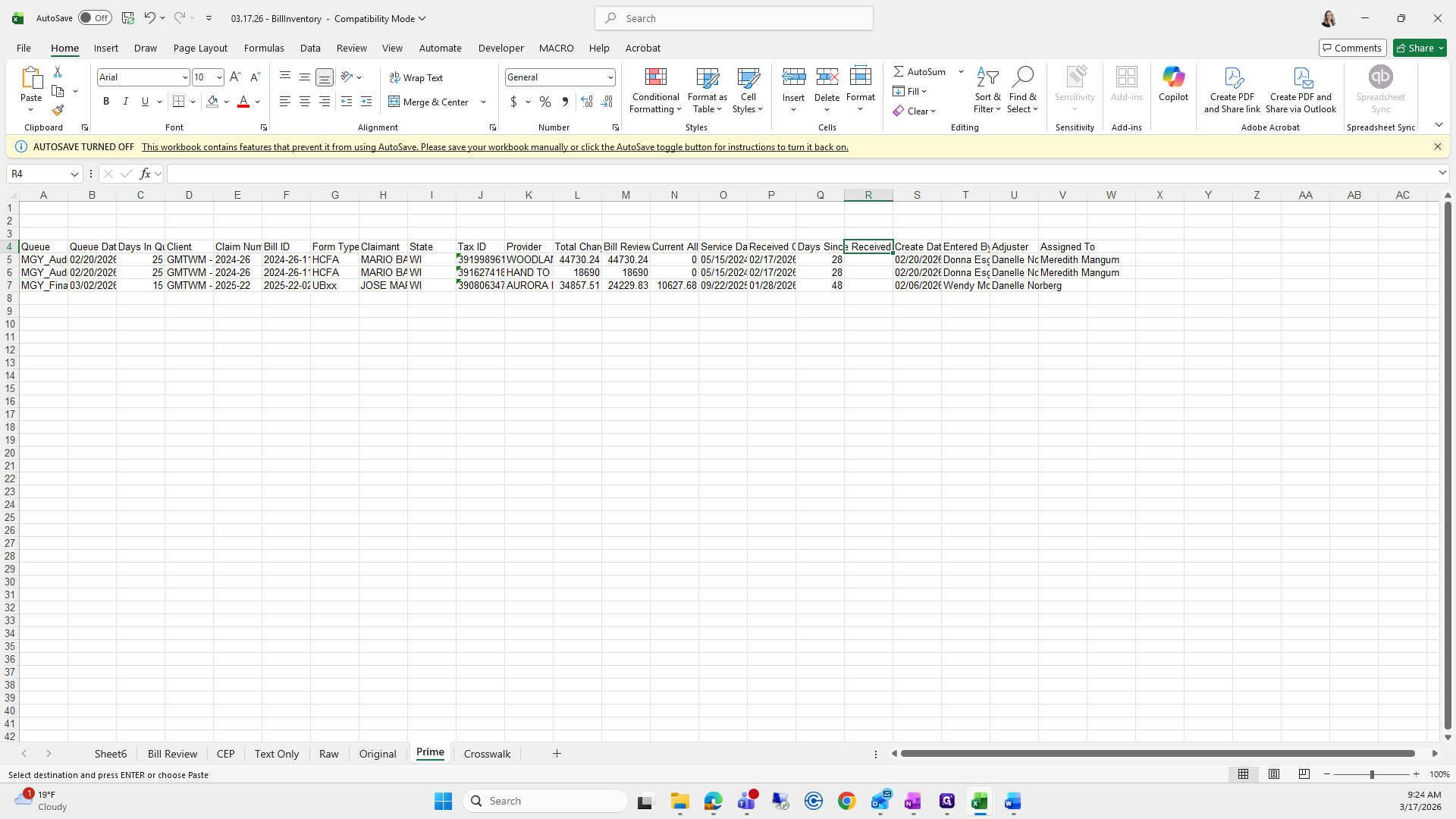
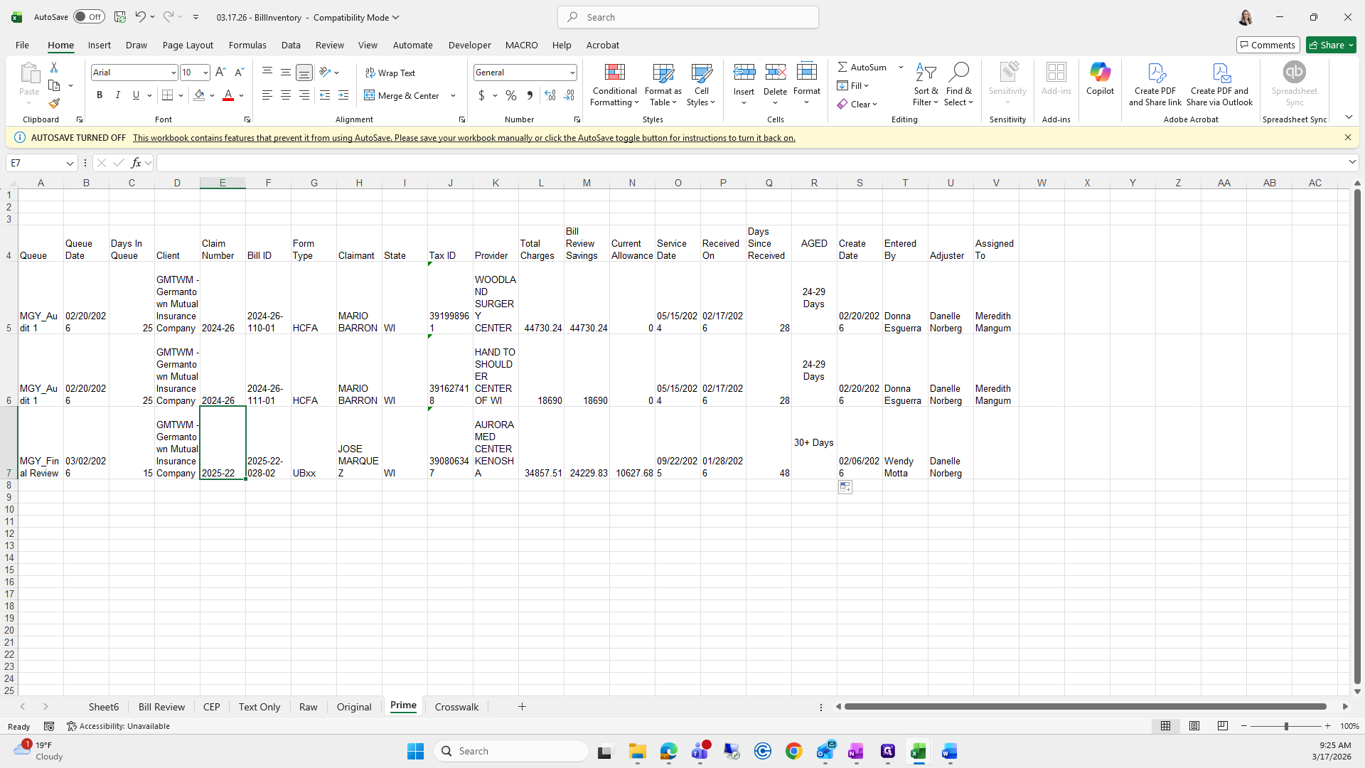
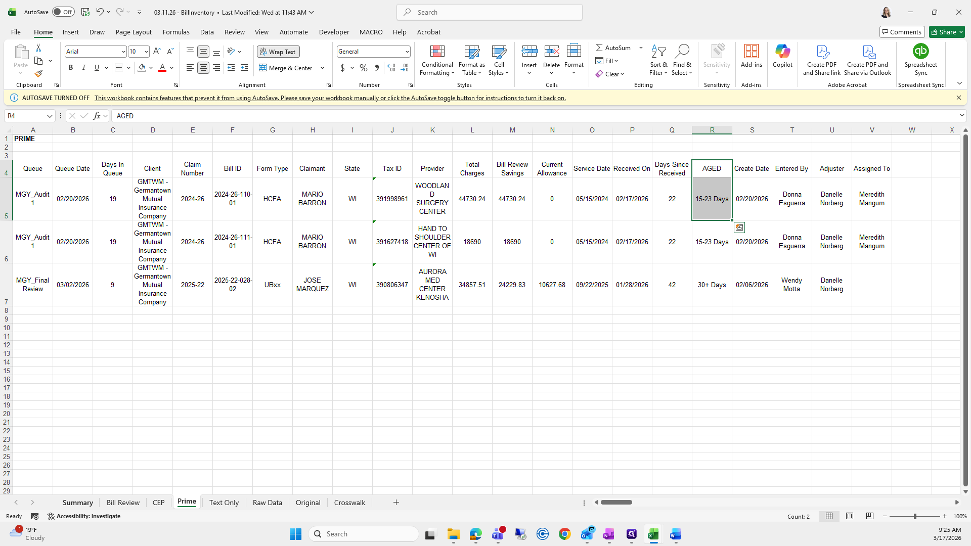
We will add a tab called Prime.
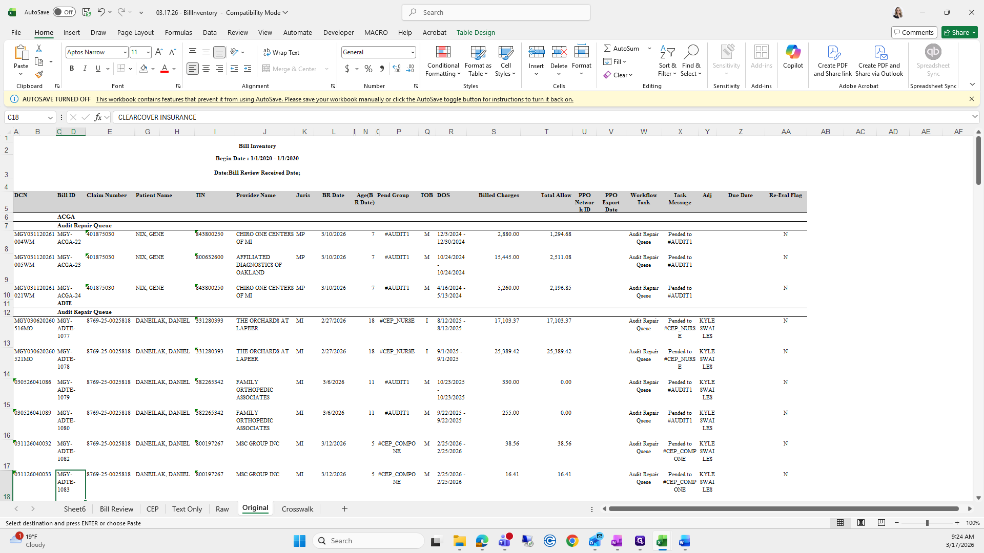
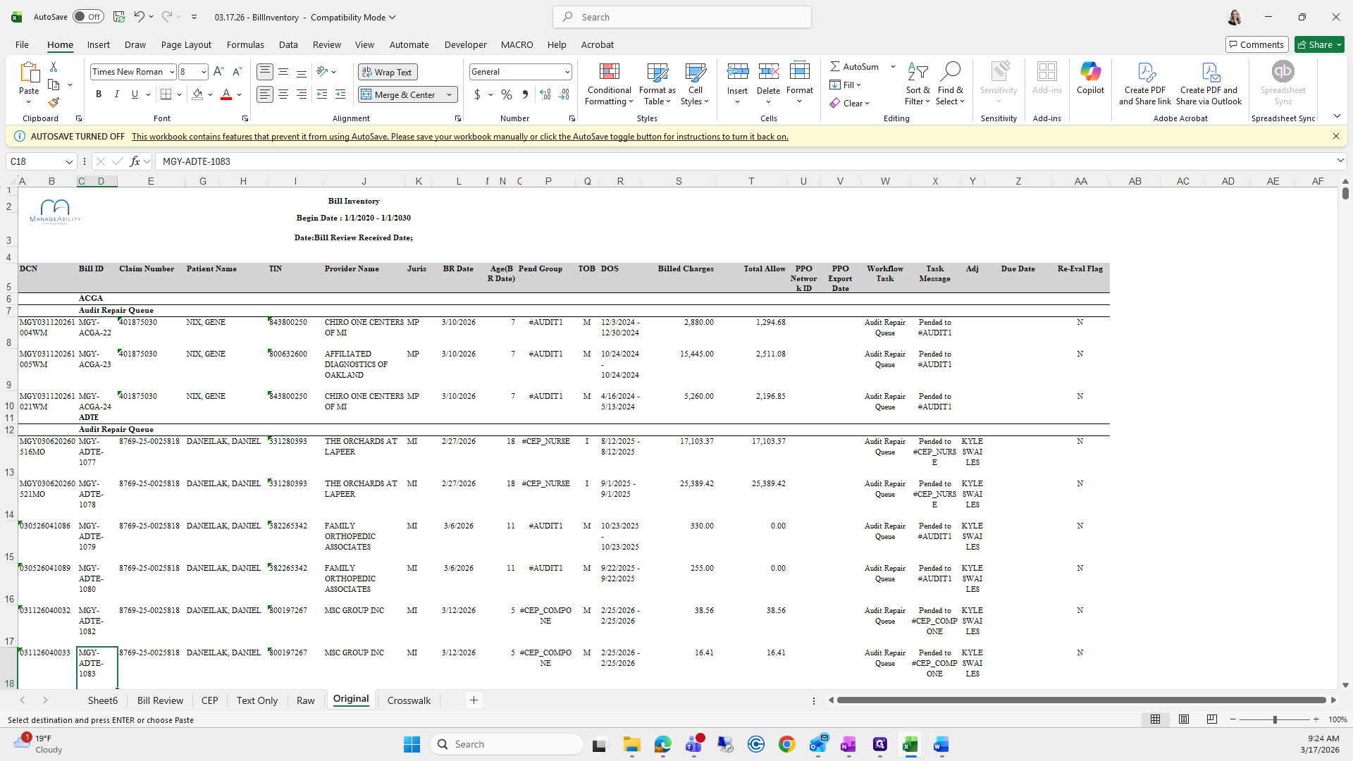
We need to make sure we paste this starting at A4, because the previous week's workbook has a formula there.
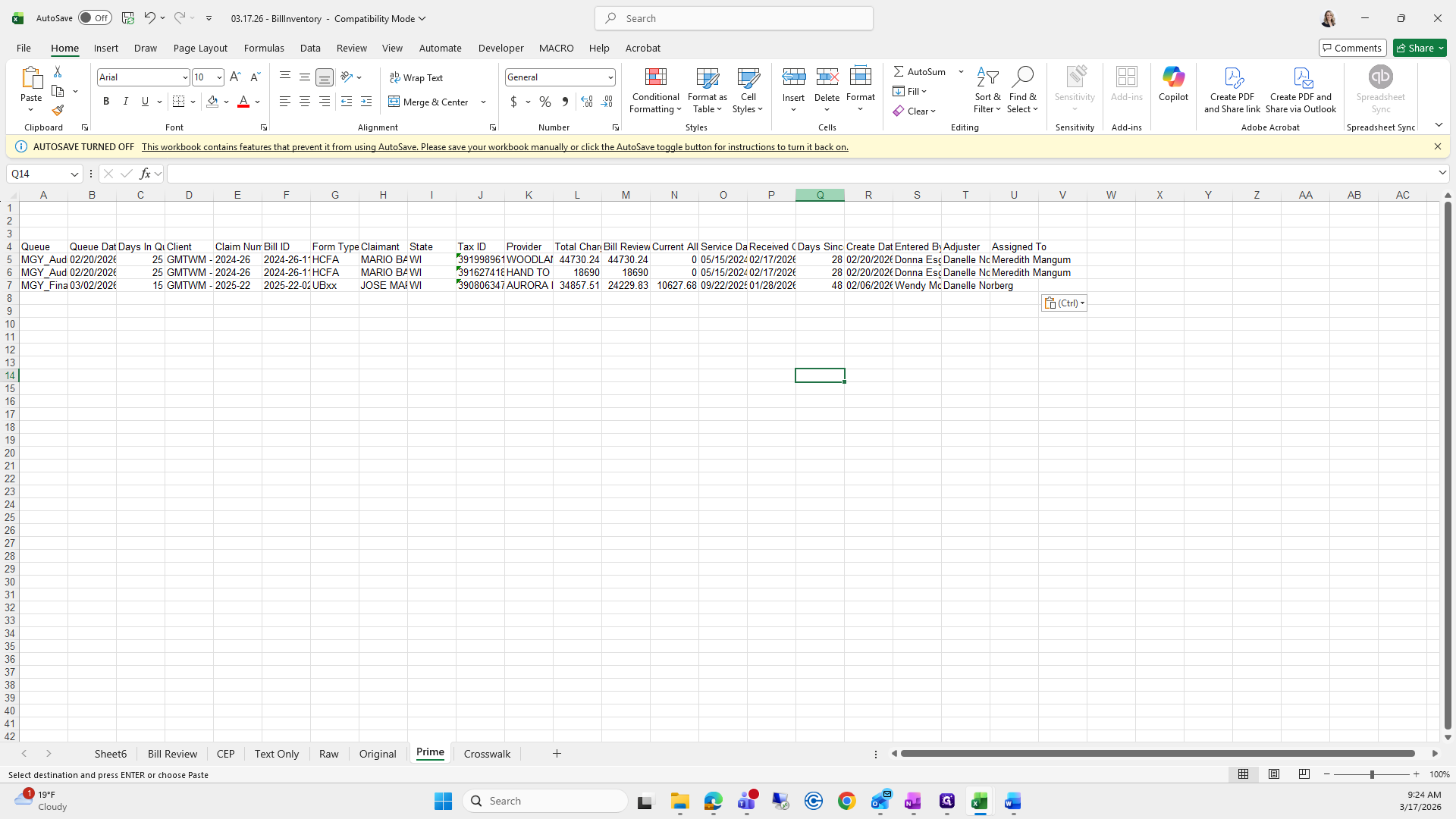
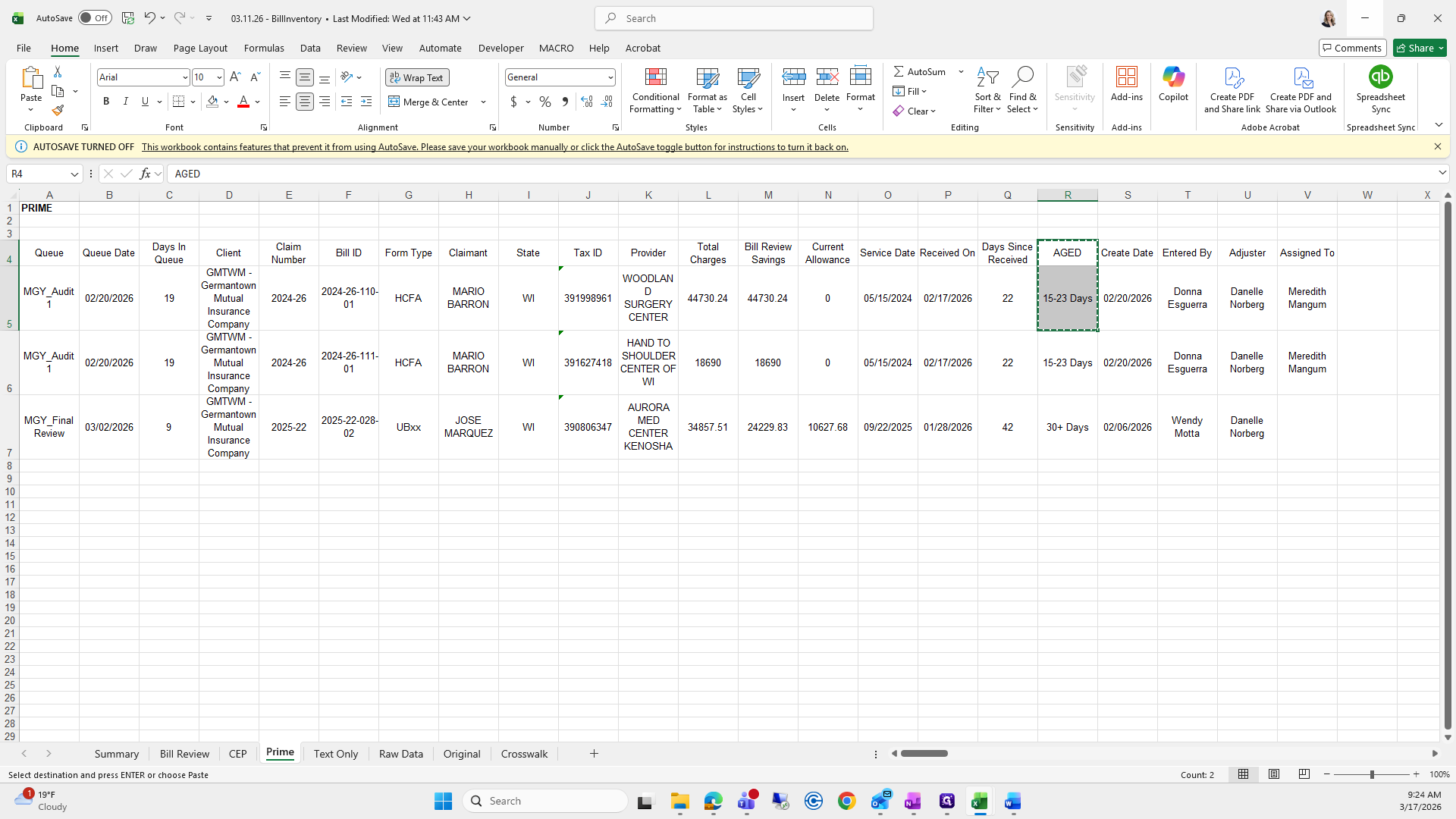
Next, where it says "Column Q Days Since," insert a column.
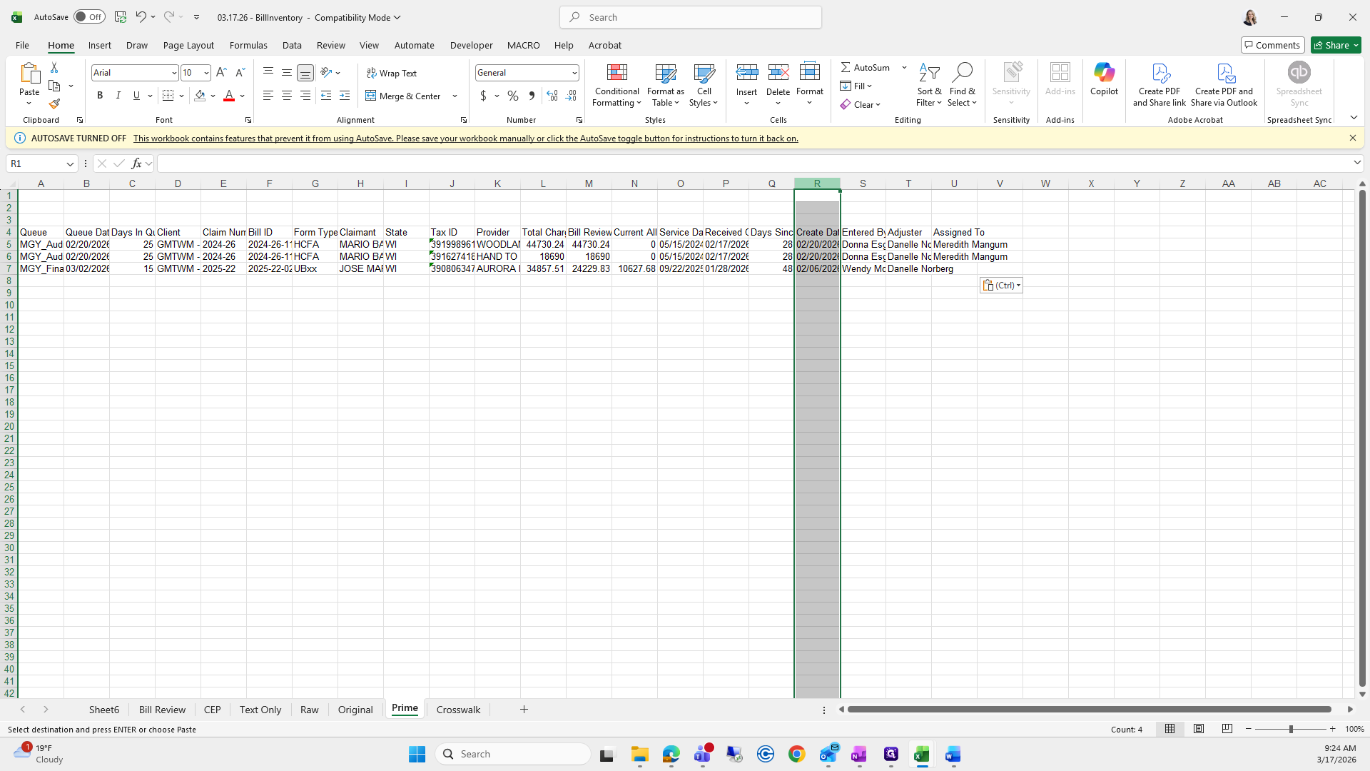
We will go back to 311, find Prime, and see the Aged in column R.

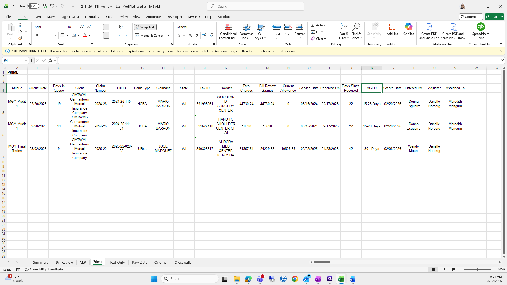
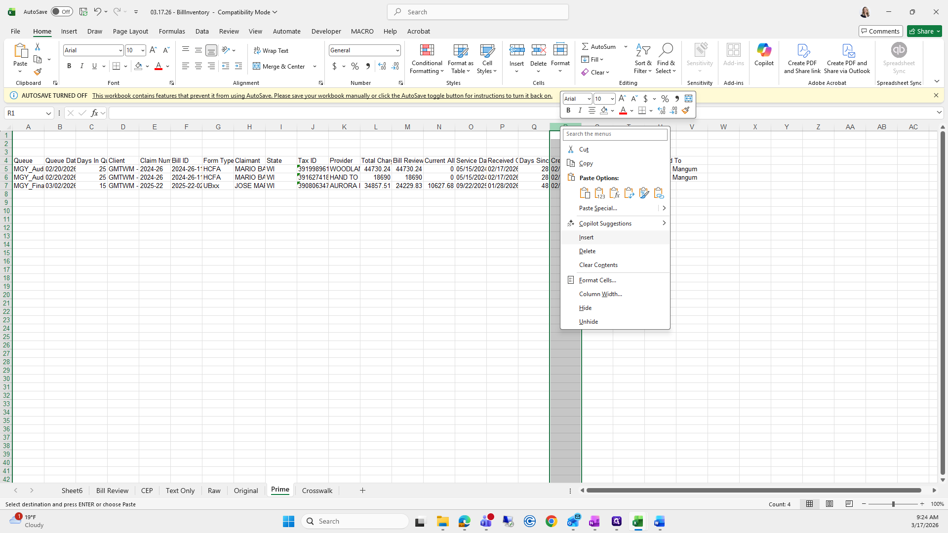
Copy and paste it. You can use wrap text if you want, but it's optional. Then, drag it down.
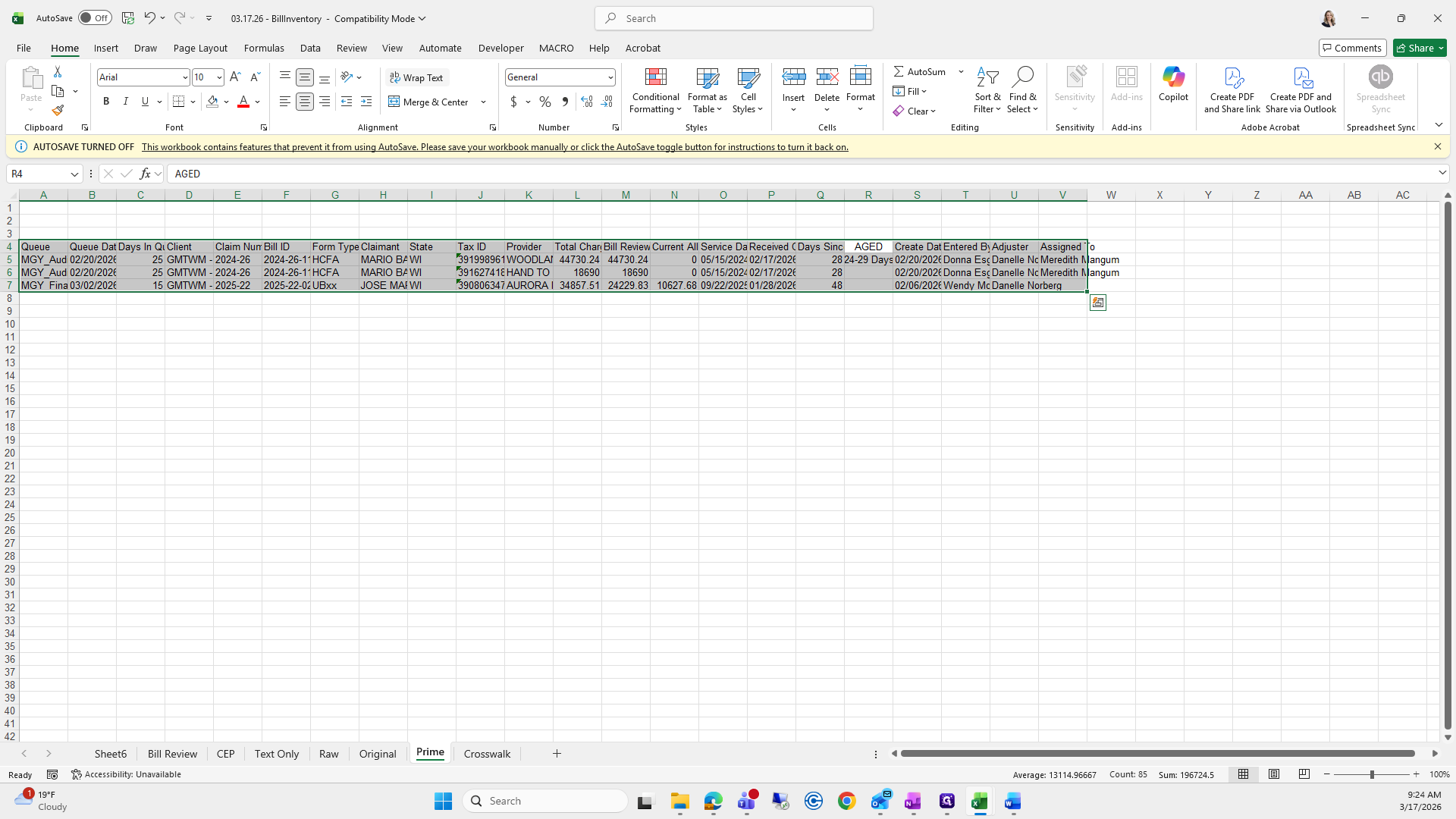
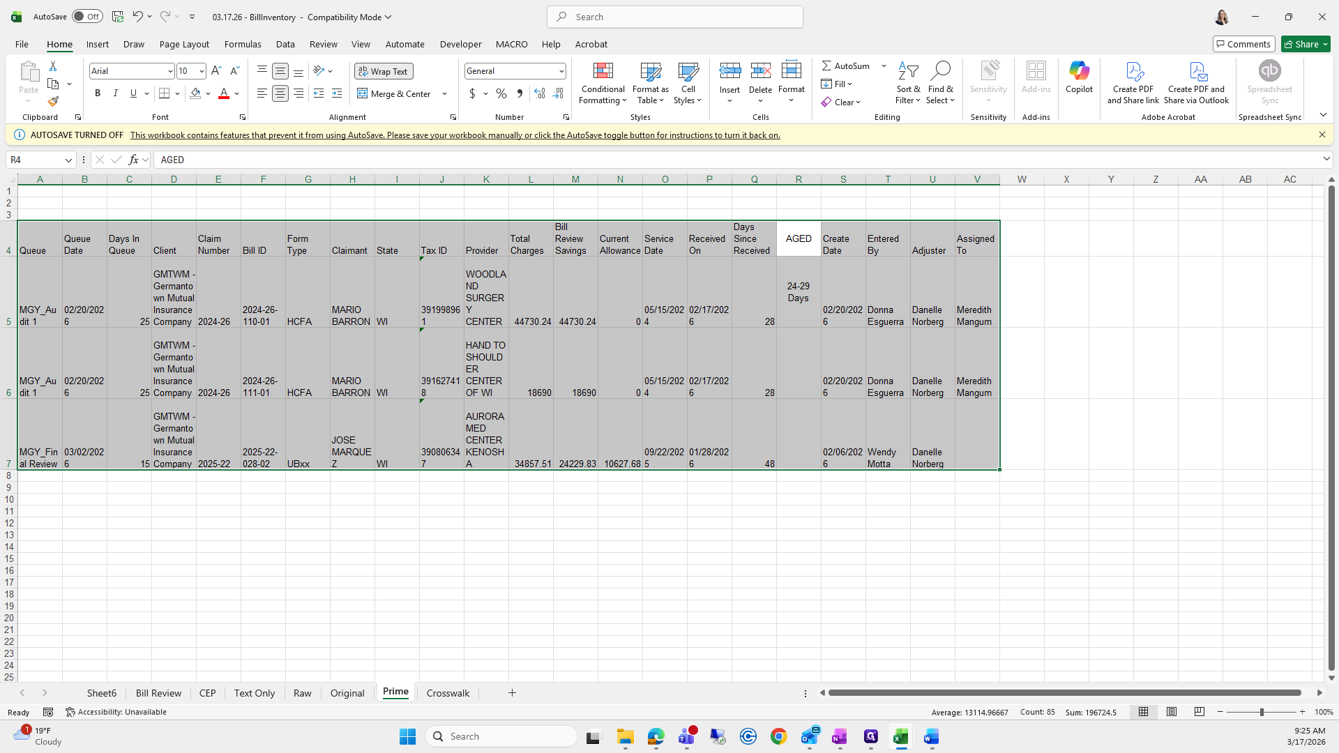

That looks good.
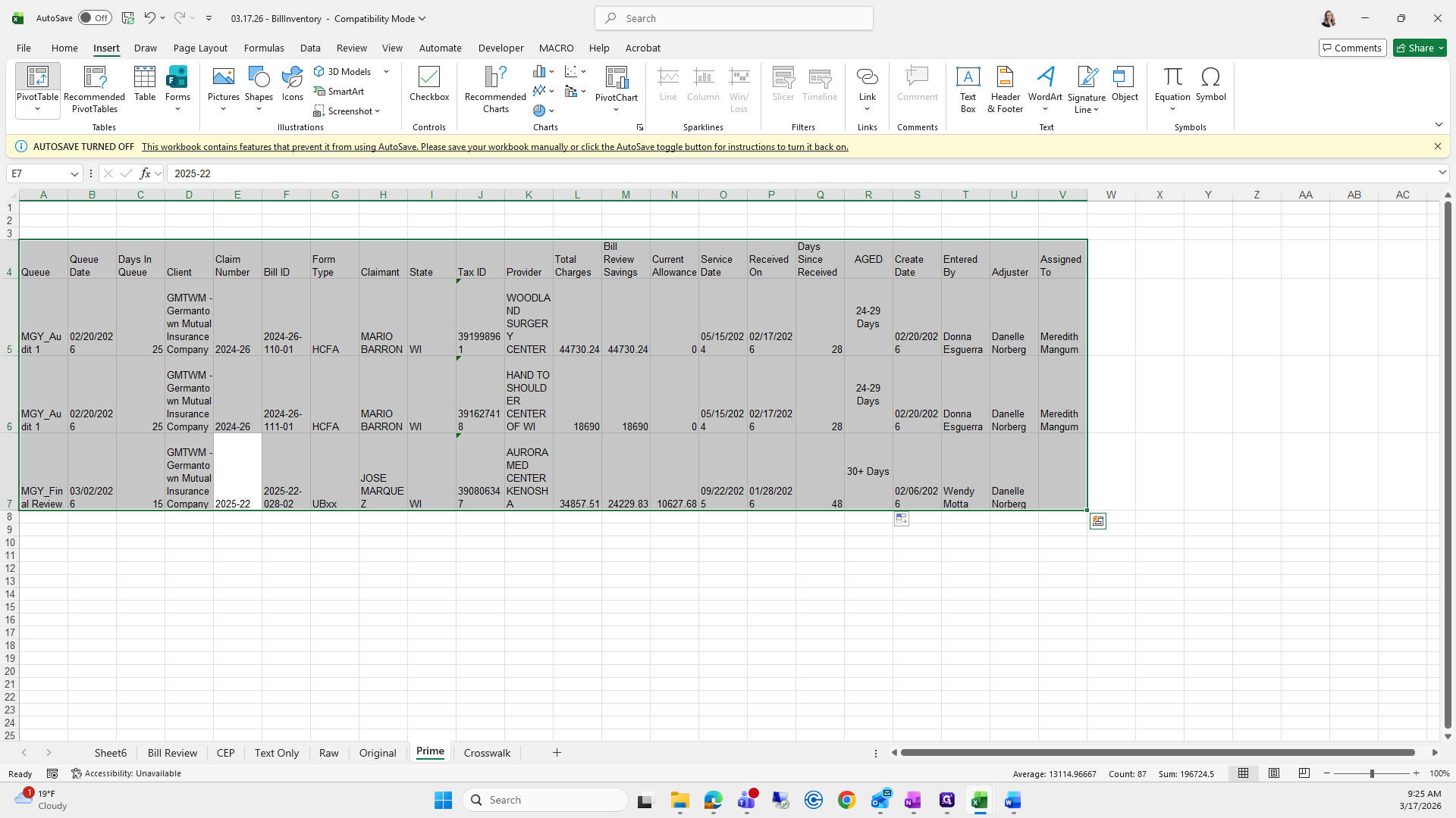
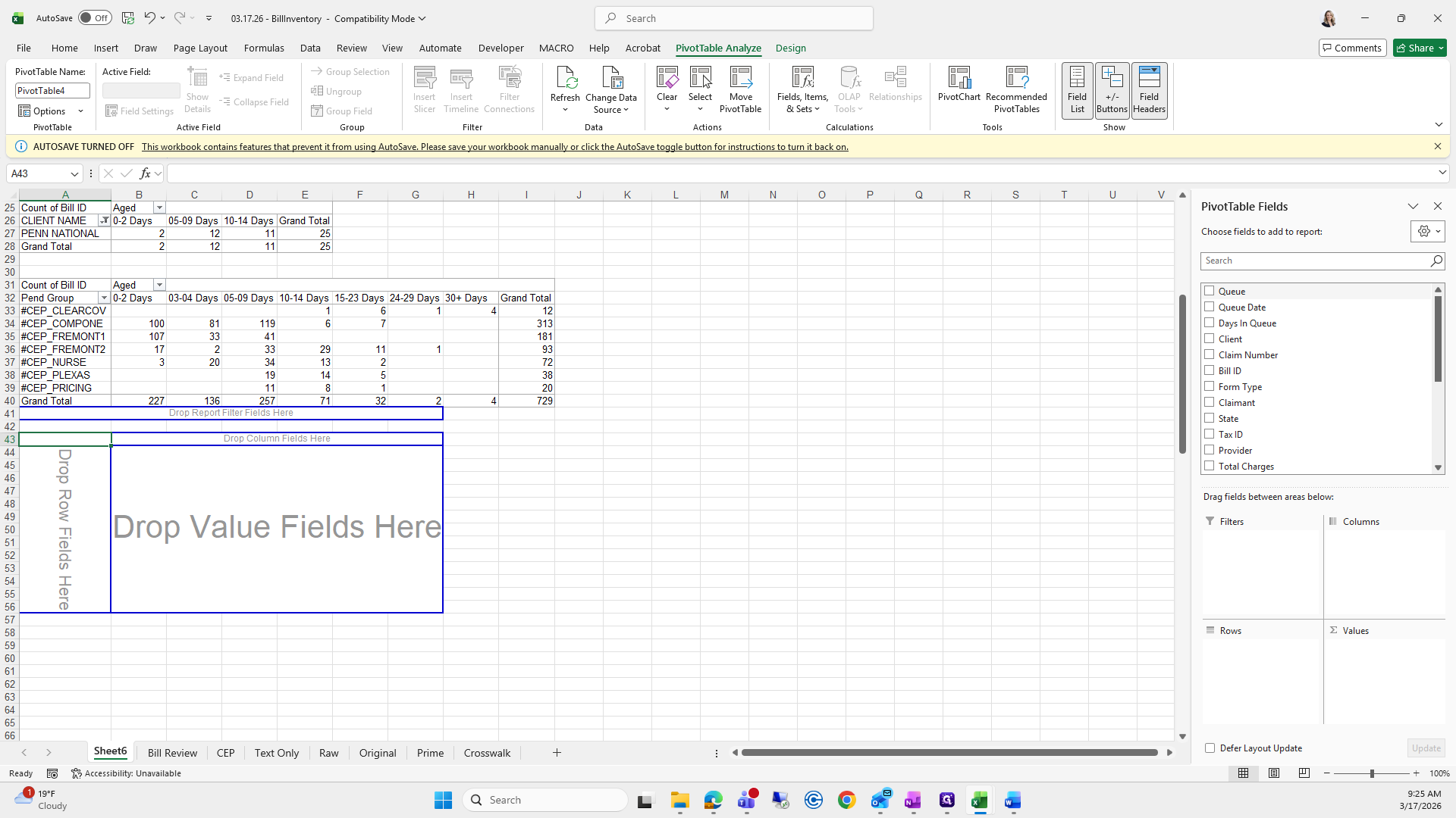
All right. Now we will create a pivot table for this.
Select All, then Insert a Pivot Table in the Existing Worksheet.

I was trying to move it.
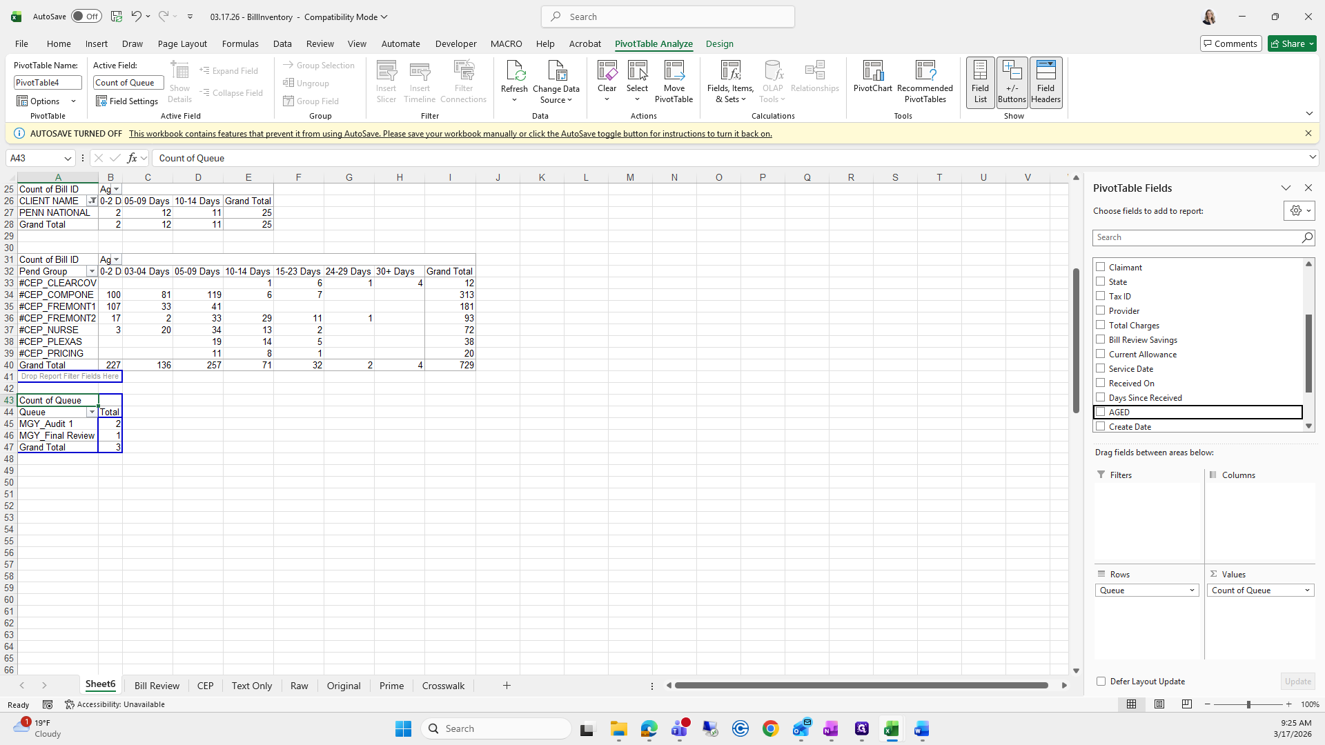
Copy, then go over here and press Okay. Next, go back to 311, check the Prime fields, and note that they are Aged, Q, and Q.

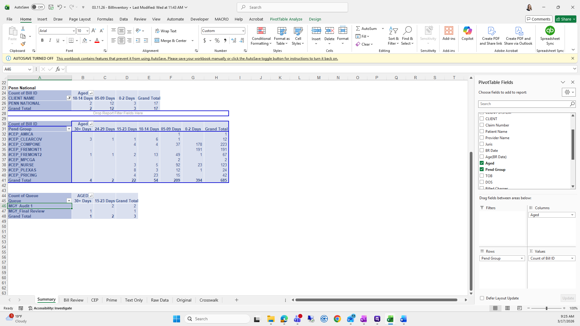

Aged in Columns, Q in Values, and Q in Rows.
Easy enough.
Aged, Q, and Q, where is Aged?
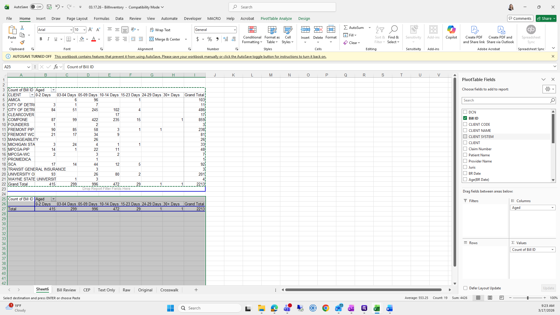
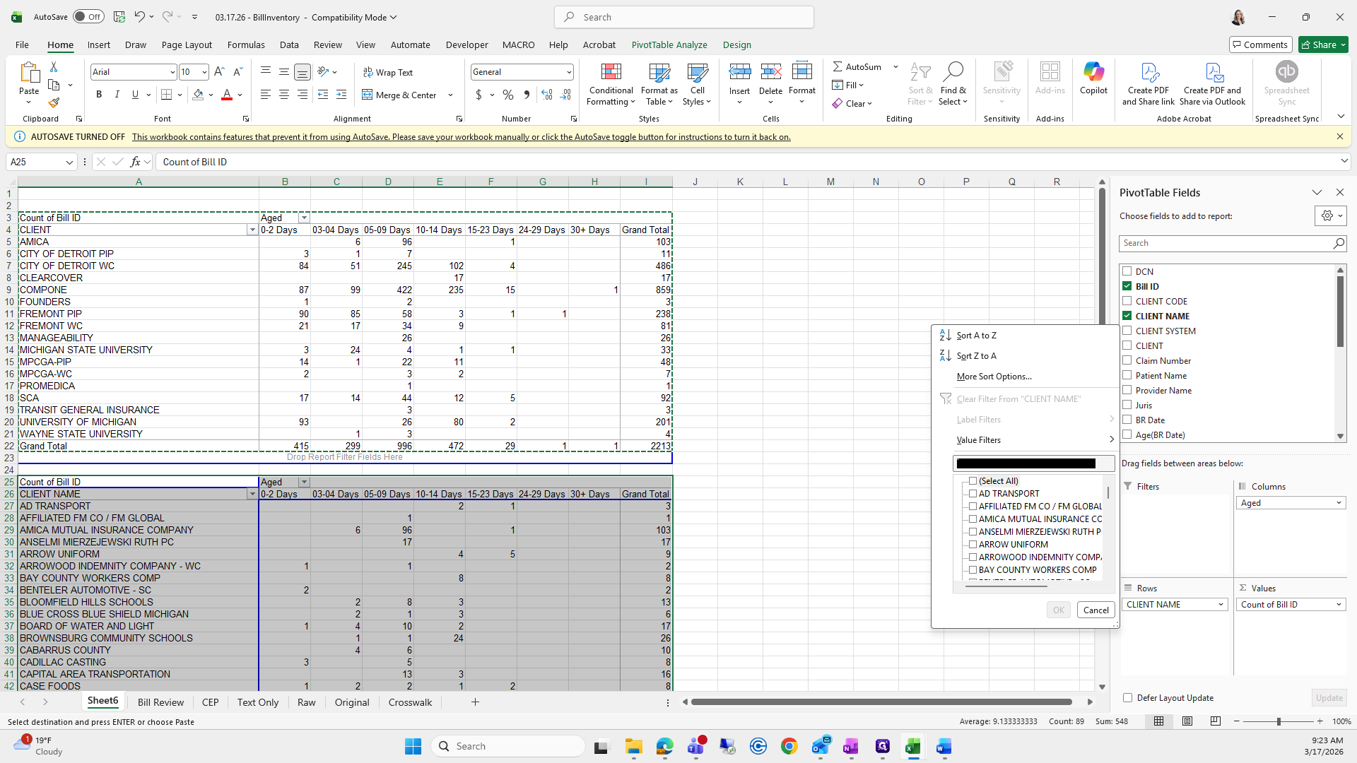
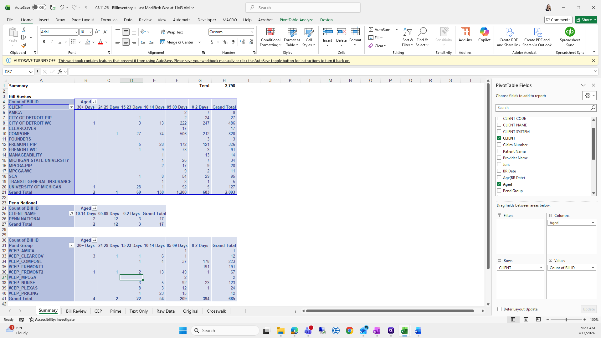
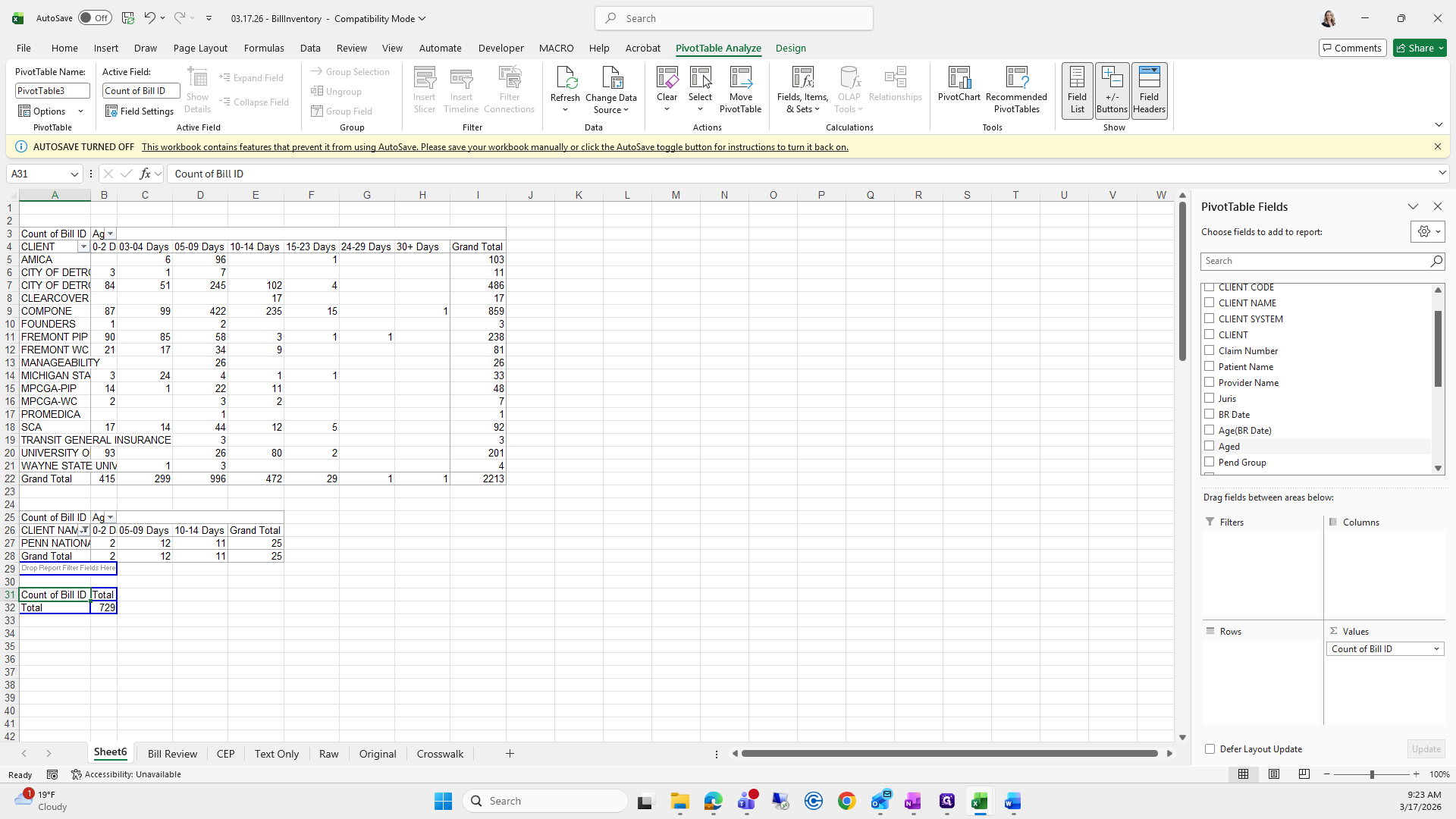
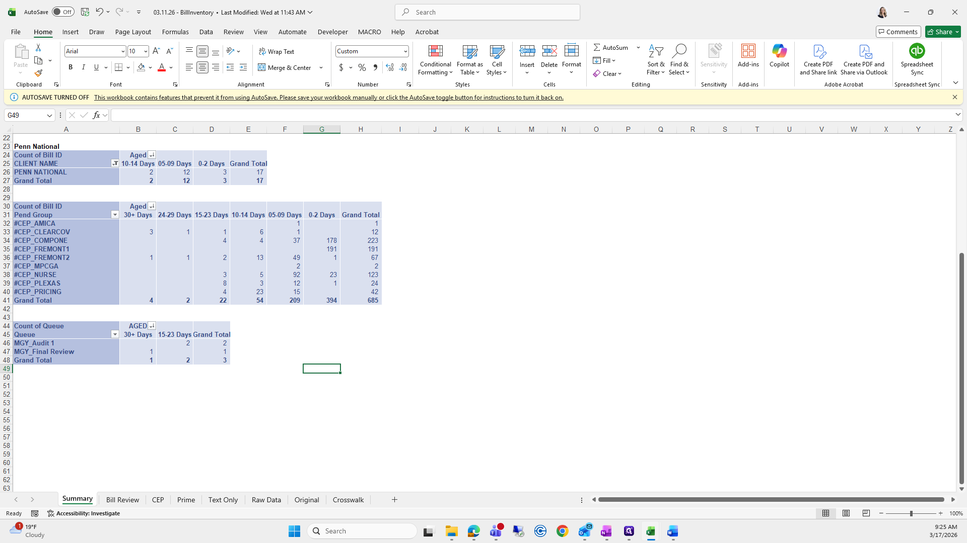
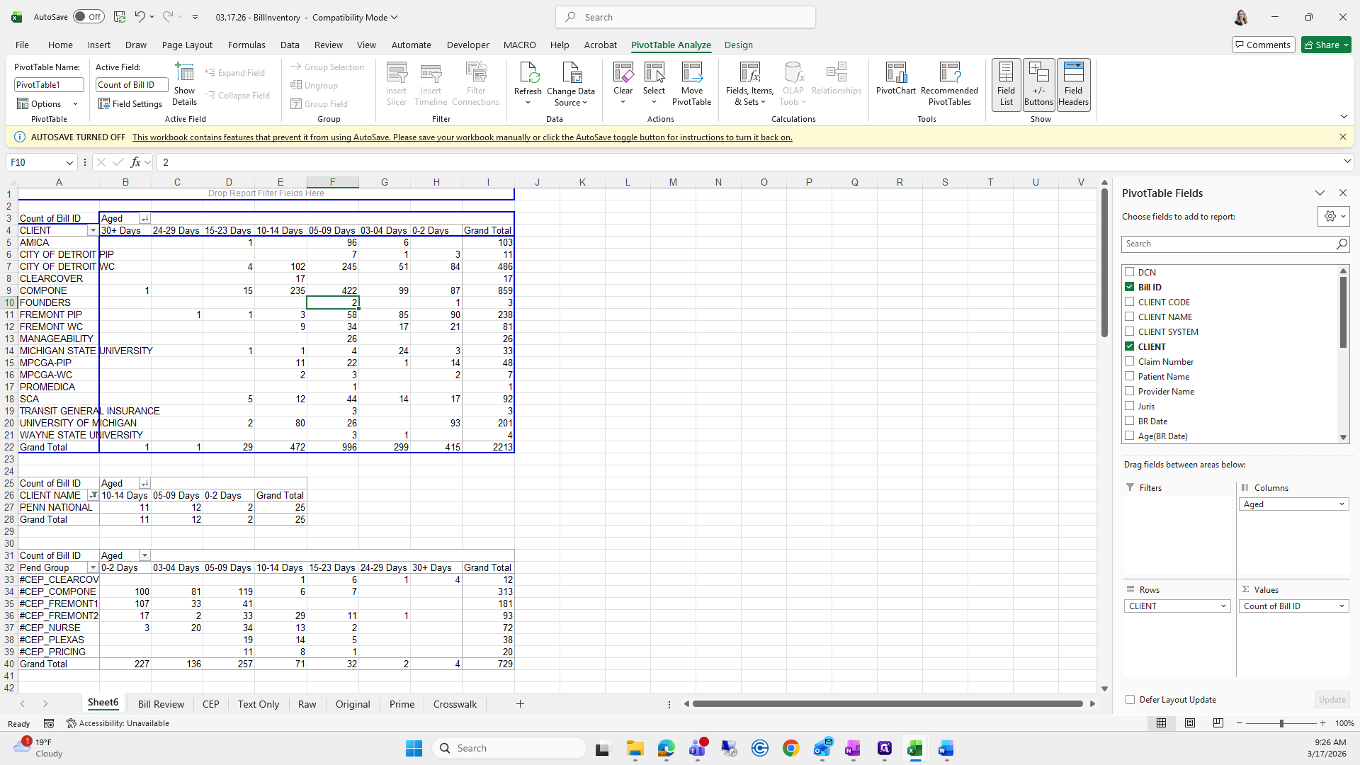
Okay. This looks good. Next, make sure all of these are set from 30 days to 2, starting at 30, since they are currently set to 2.
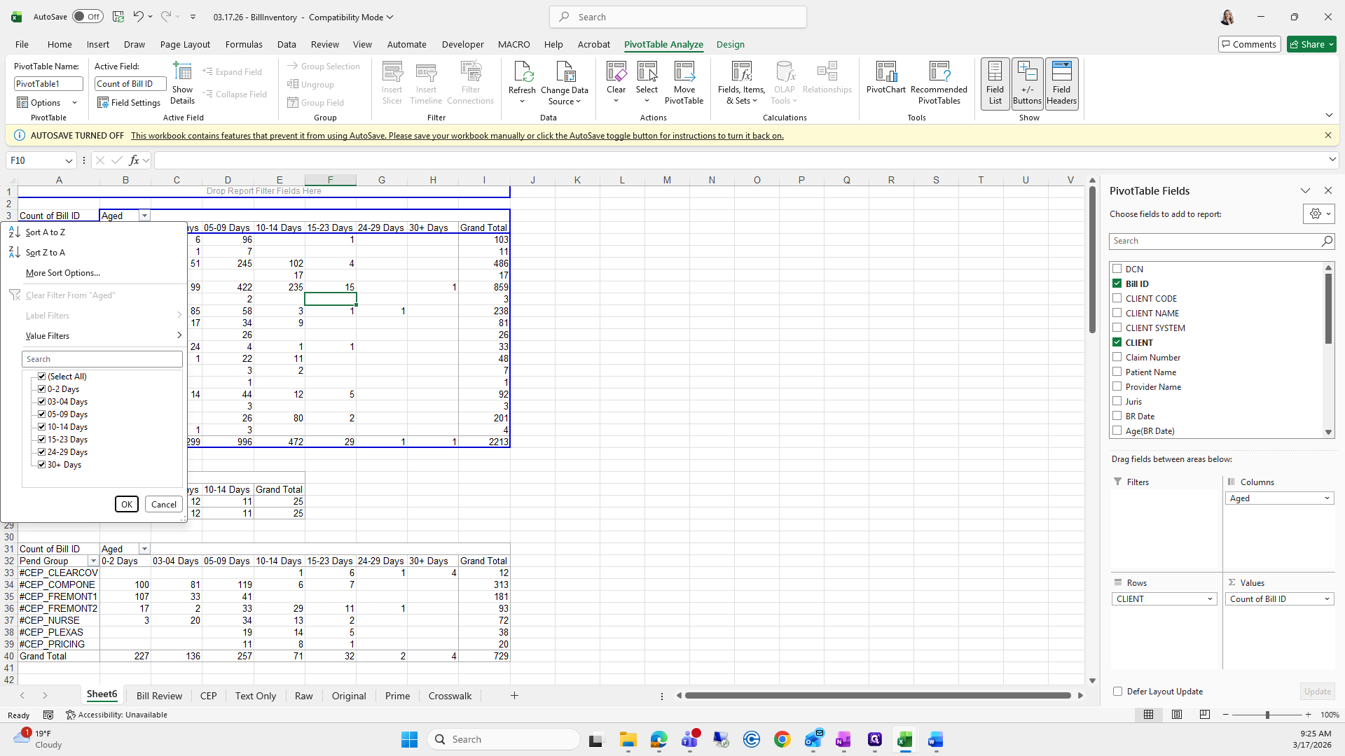
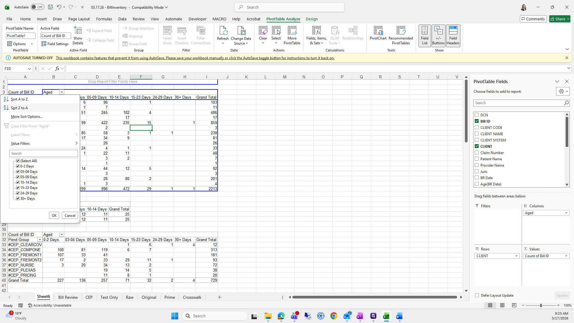
To do this, click the H dropdown, select "Sort Z to A," and press OK.
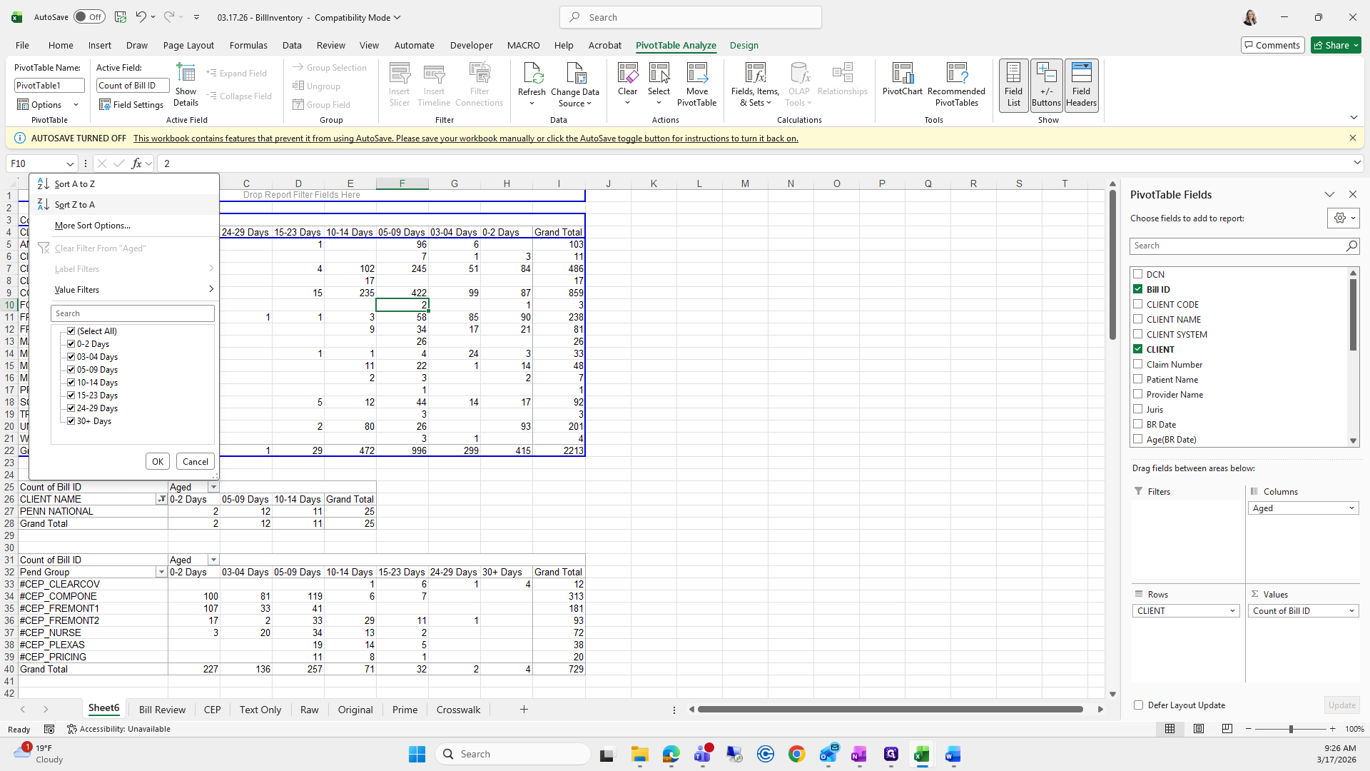
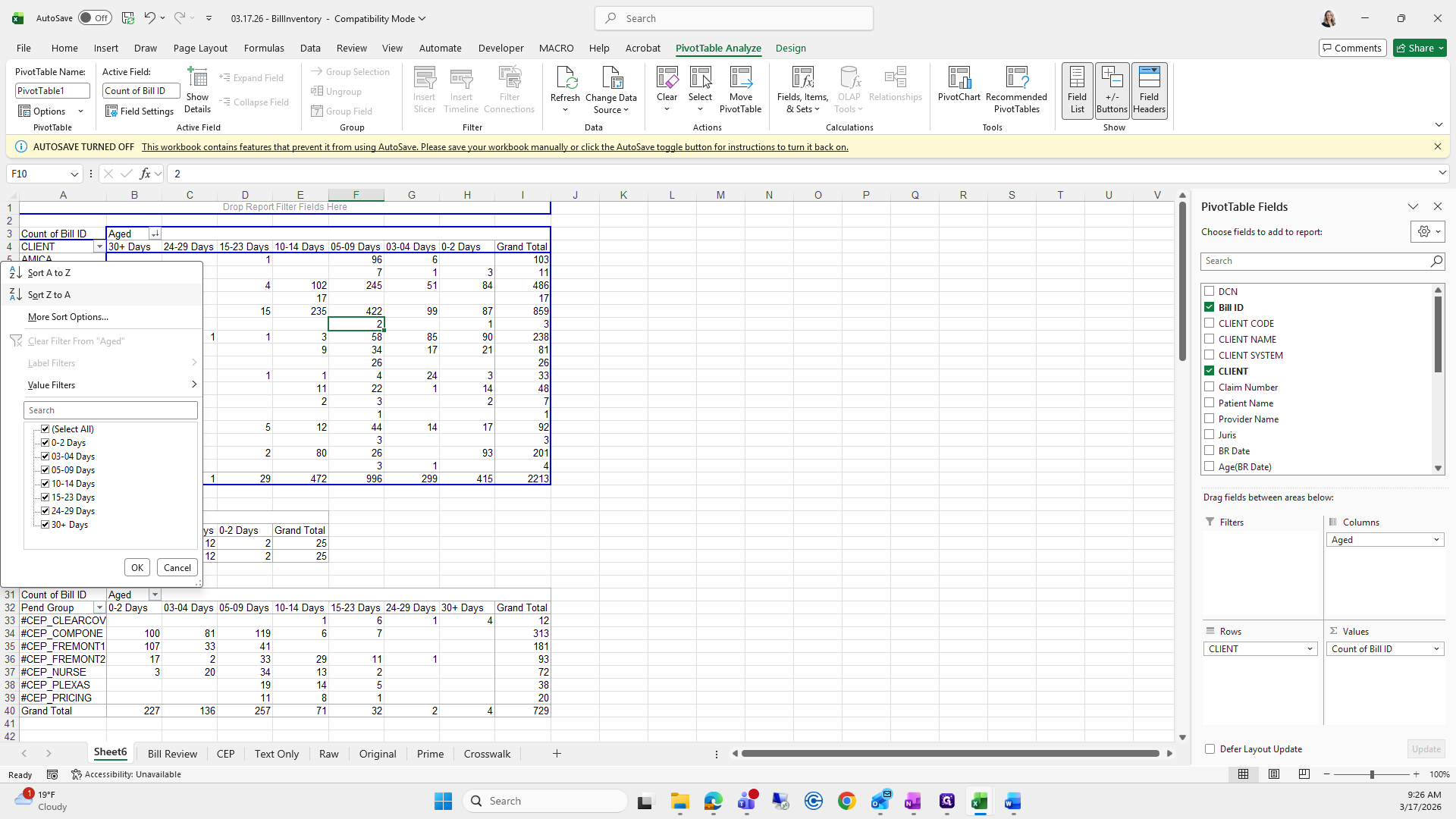
Do that for each pivot table.
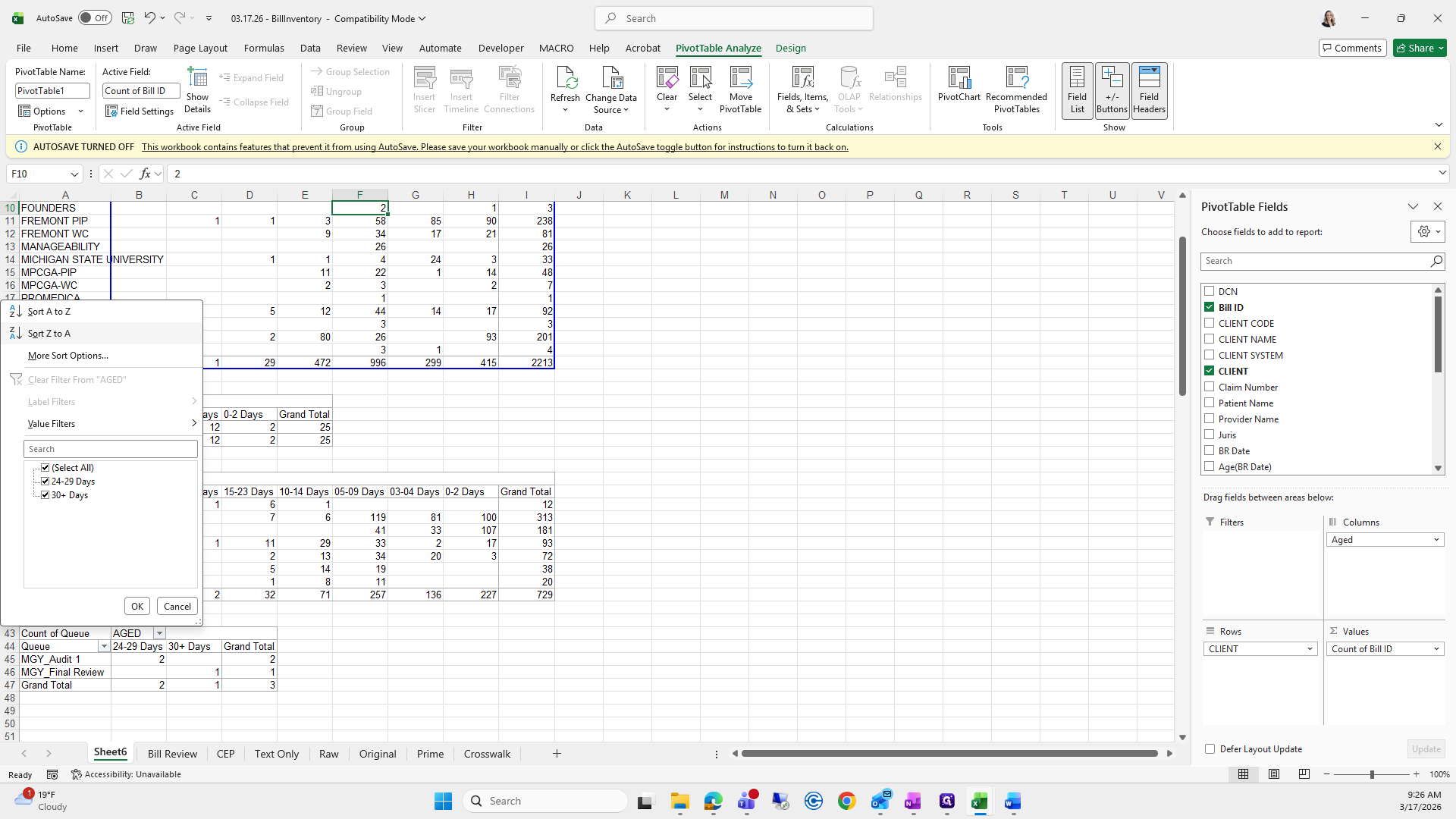
Z to A, Z to A, Z to A, Z to A.
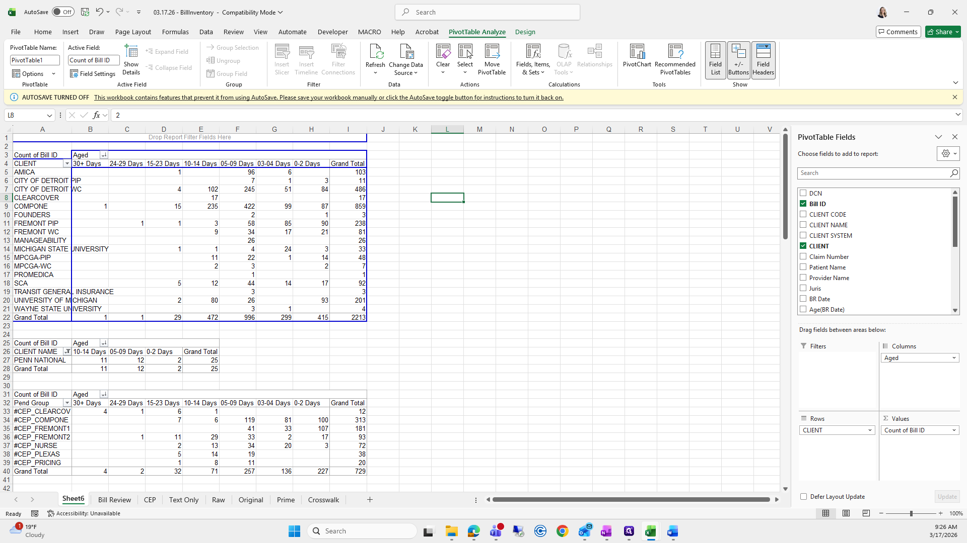
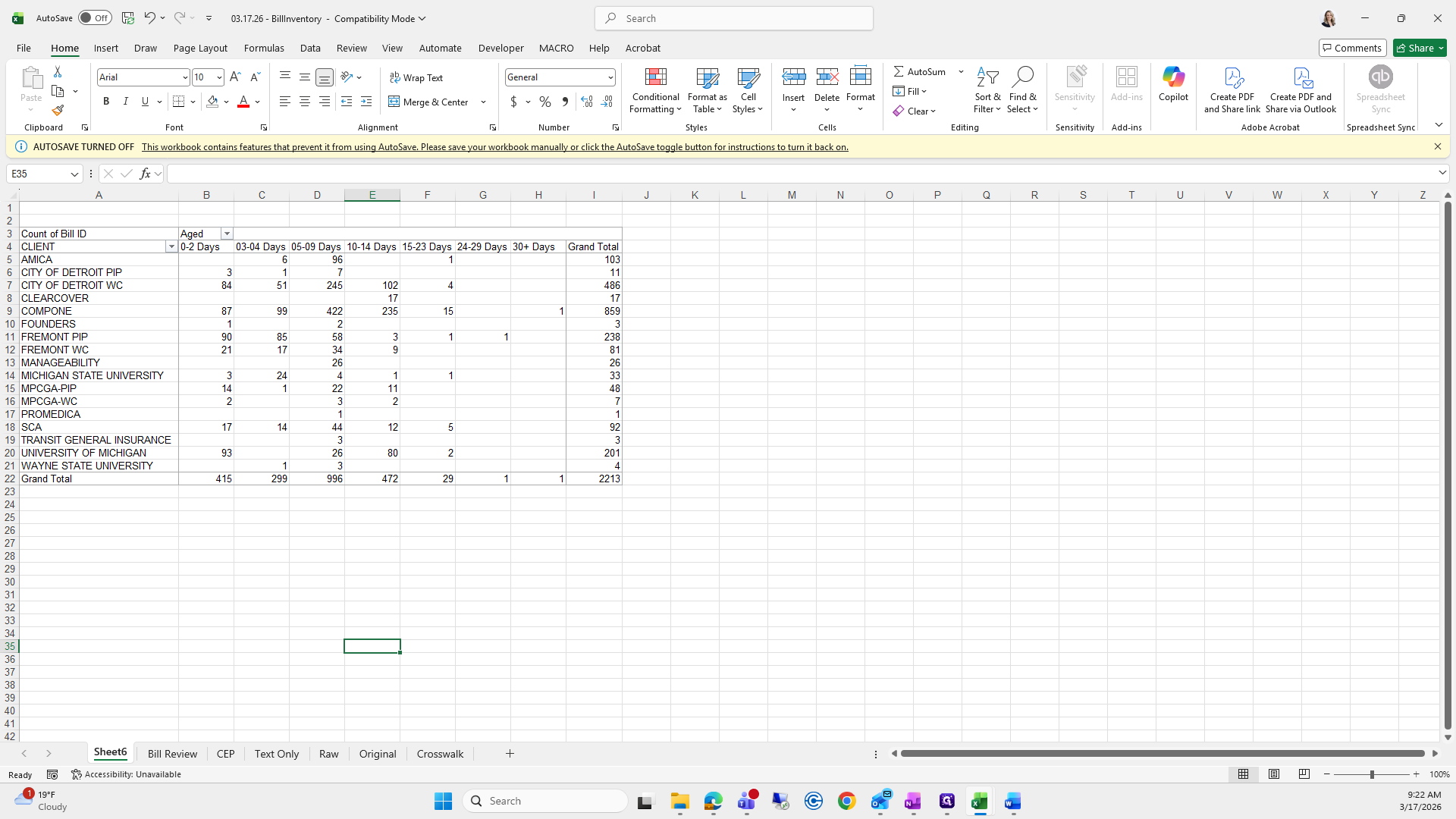
That looks good. And then a quick formatting.
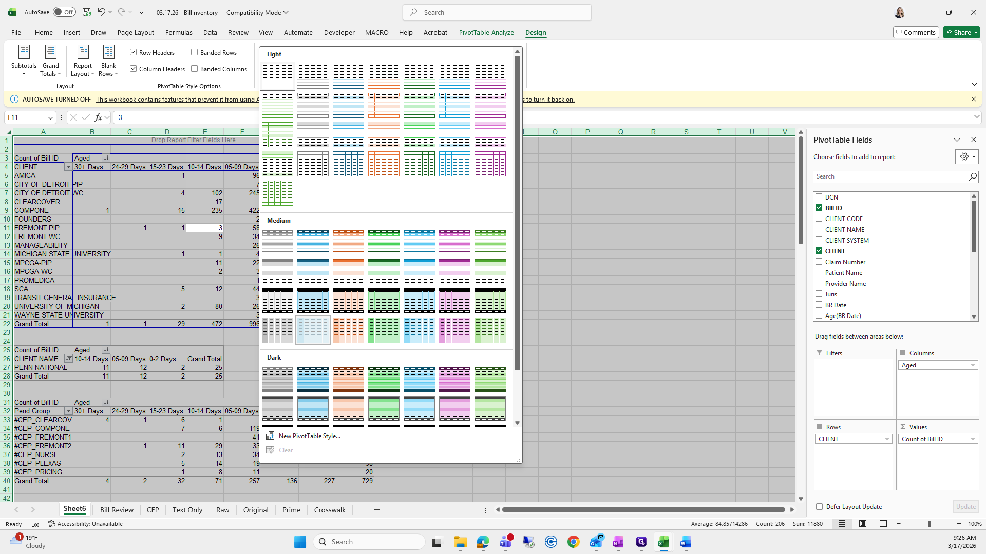
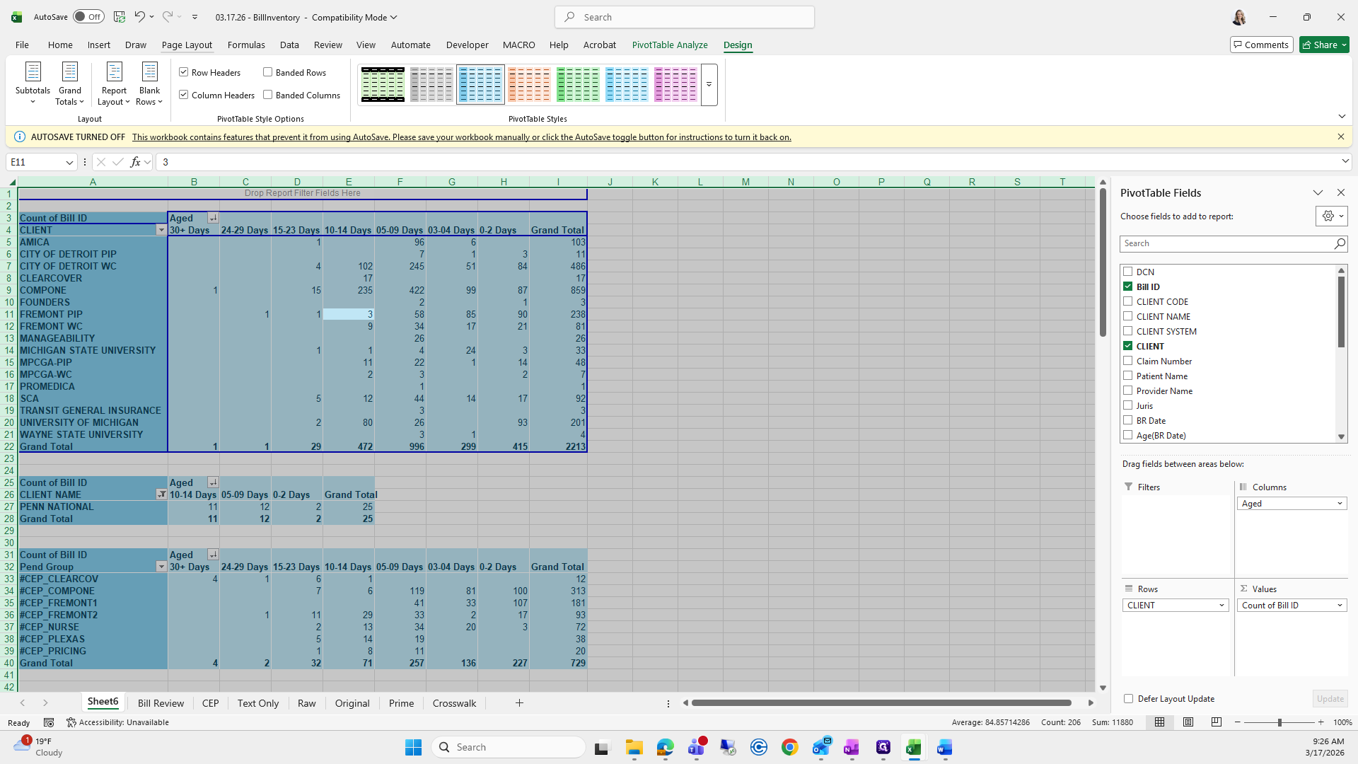
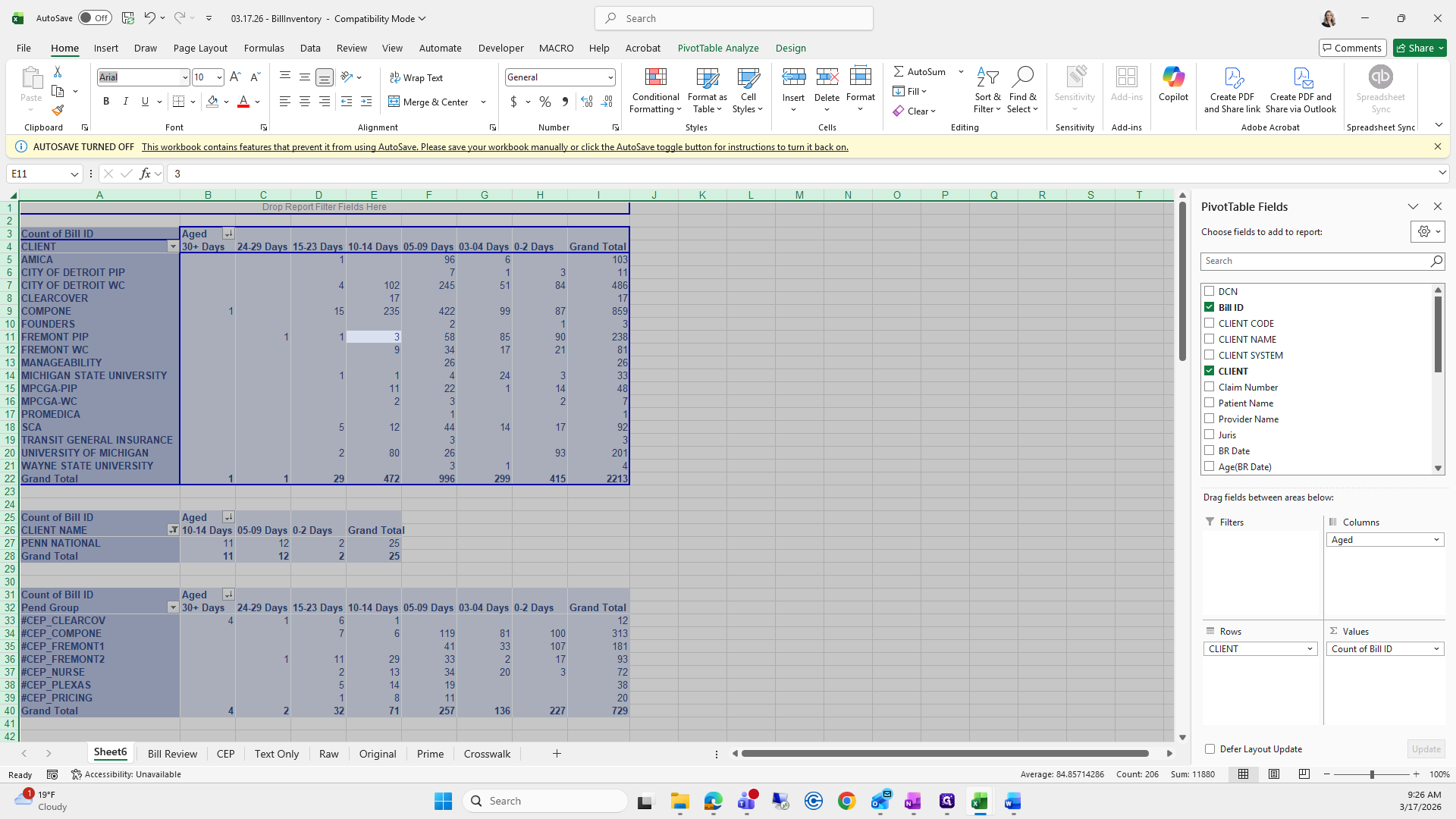
All I do is select all.

Select All, then choose Design.
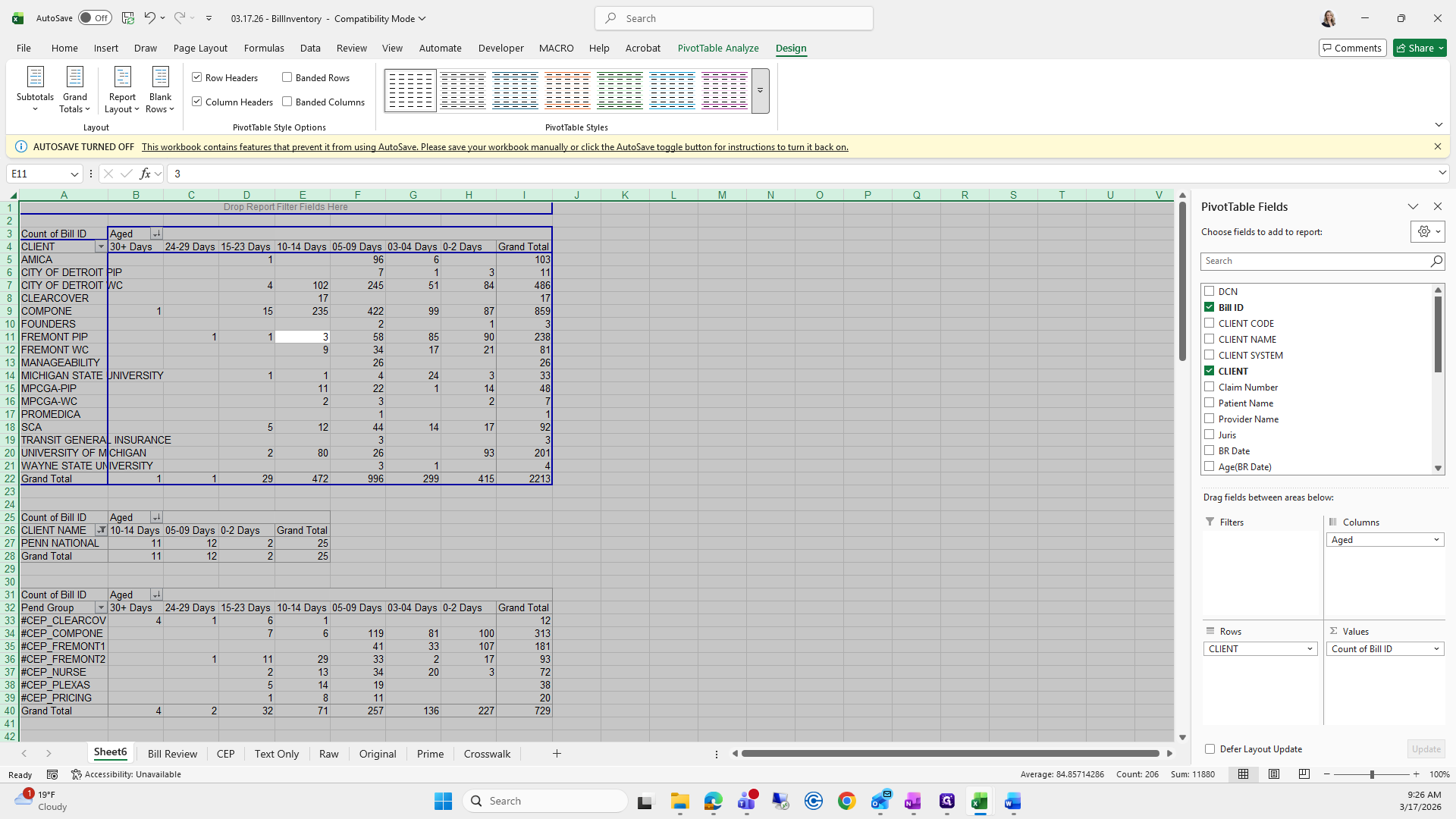
I usually choose this one.
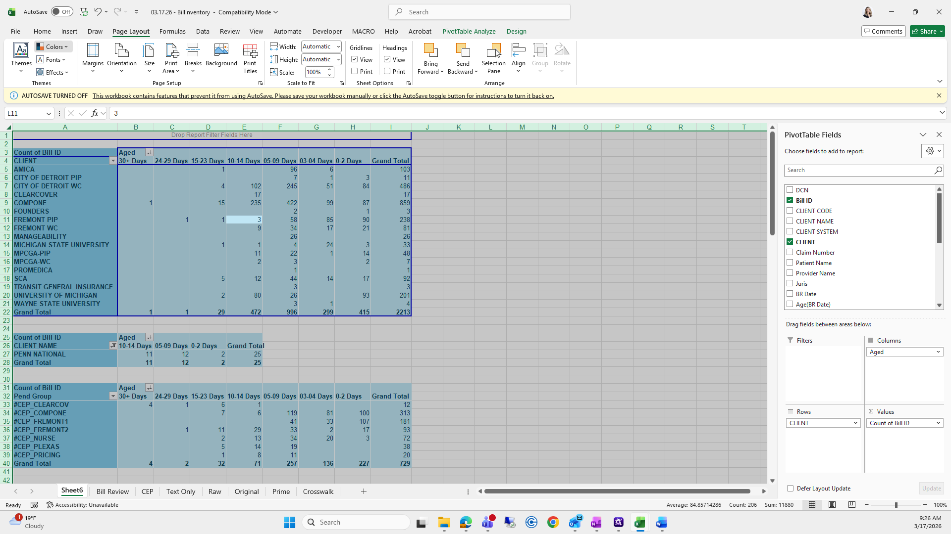
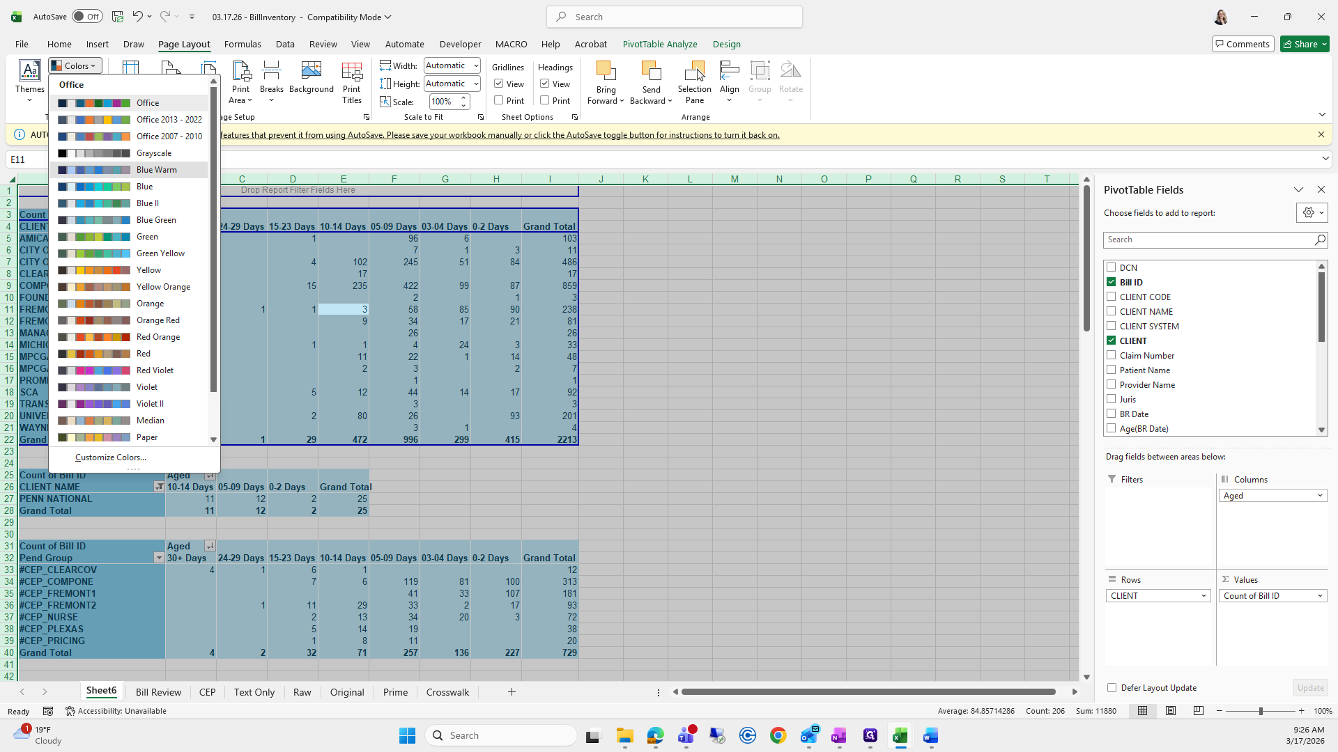
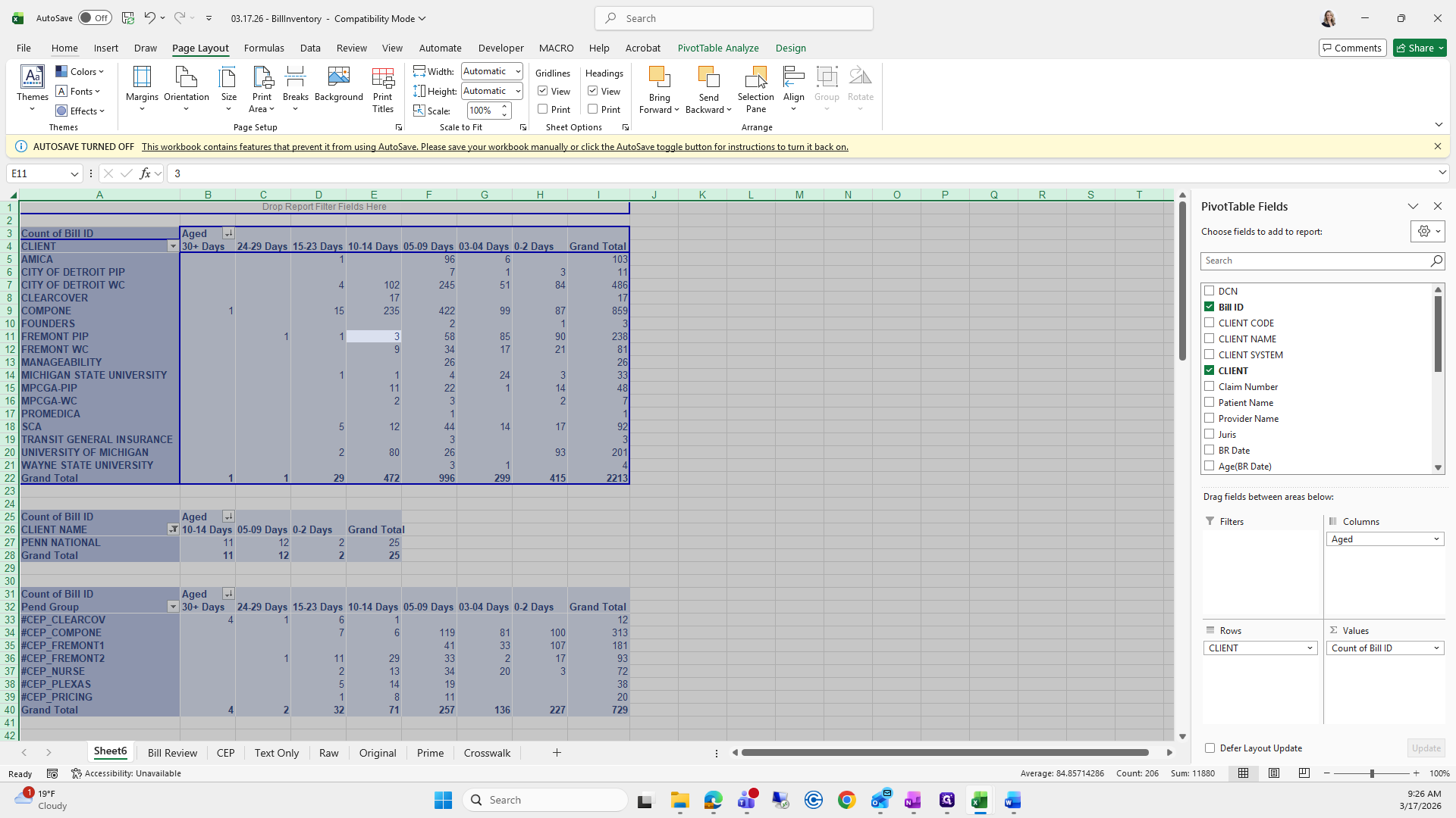
Page Layout, Colors: I use Blue Warm. I also like to change the font, but you can keep it on Arial.
It does not matter. This video will end soon, so we'll make a fourth one since it only allows five minutes.