A guide for checking agent Yannick2
Step by step guide for checking agent Yannick2
By Miki
1
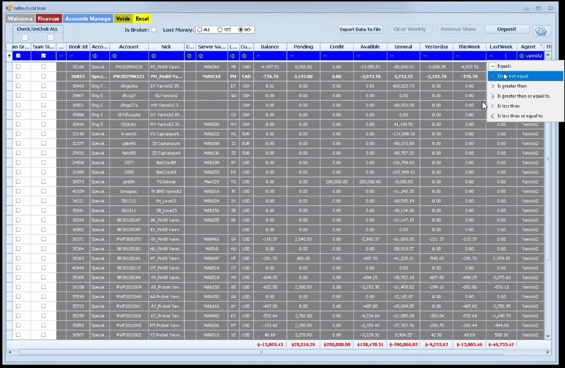
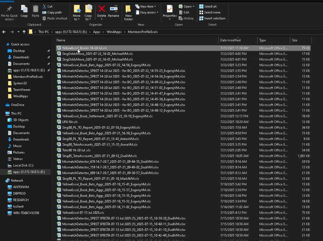
Start with Back Office file (BO), open the yellow excel file then filter by agent name "Yannick2" and filter the last PnL last week. Select "Does not equal to zero"
2
Go to weekly PnL file (Our tool) and click on Yannick2 sheet then create the template for adding data.
3
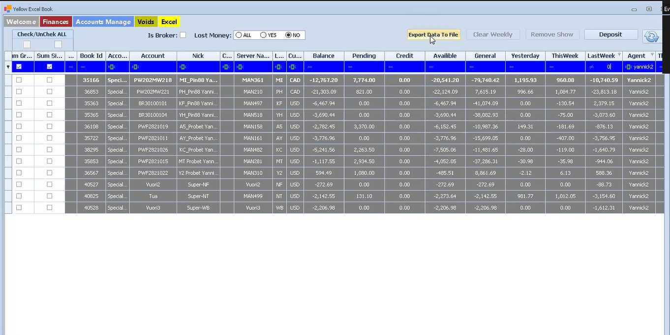
Go back to the BO then export data to the excel file by click " Export Data To File"
4
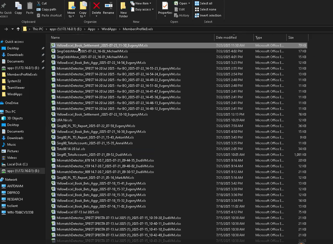
Go to the download folder, it will show the excel file that has been exported.
5
Rename the excel file to the date of last week then open it.
6
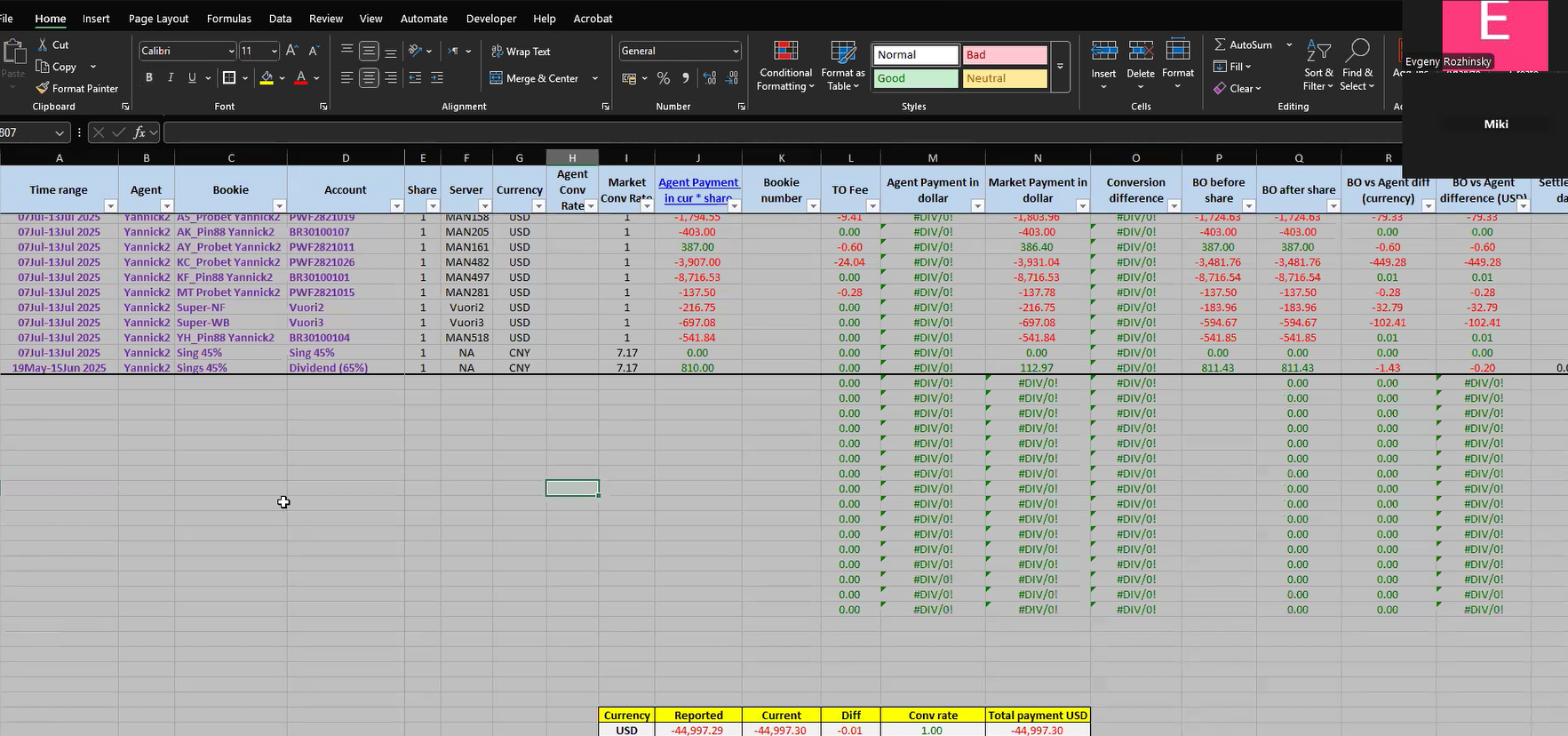
We will get the PnL data from last week, then adjust the table to make it easier to read.
7
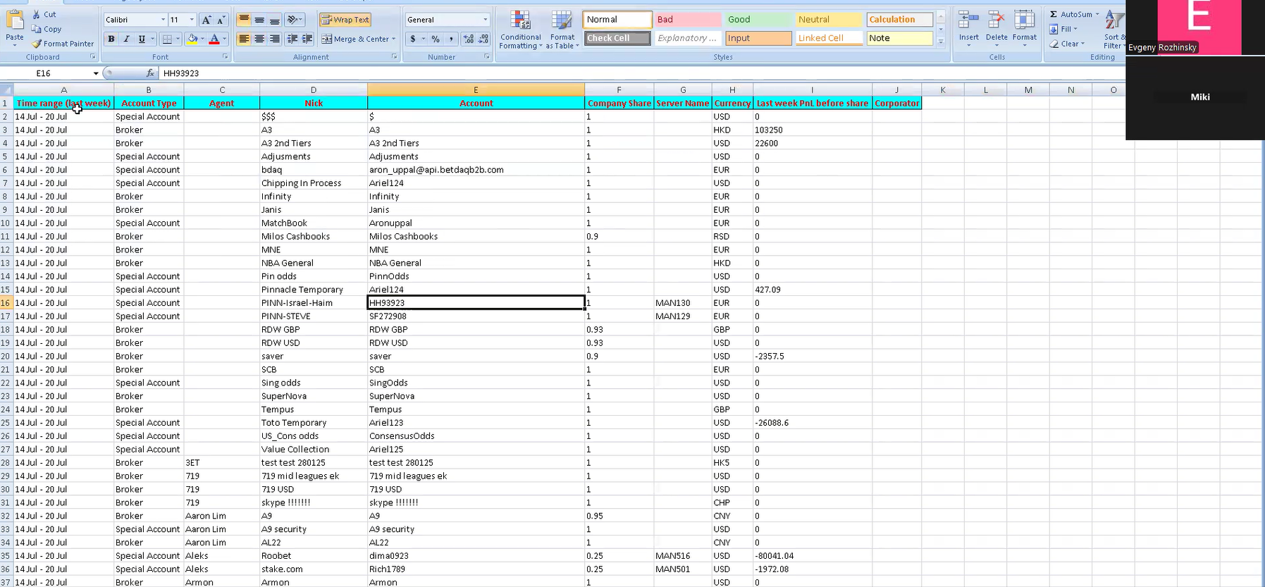
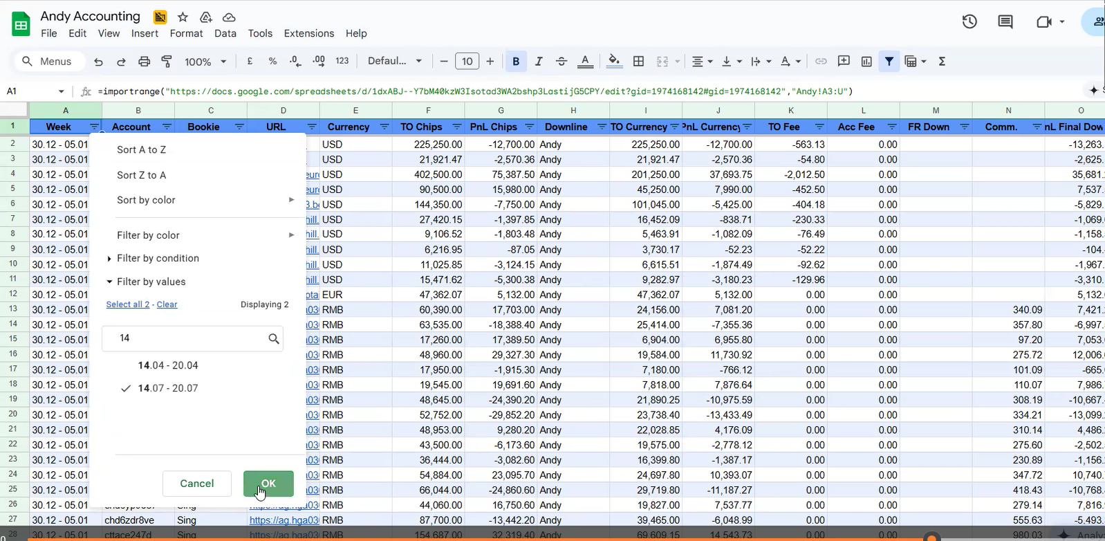
Put filtertation the titles then filter to Yannick2 agent.
8
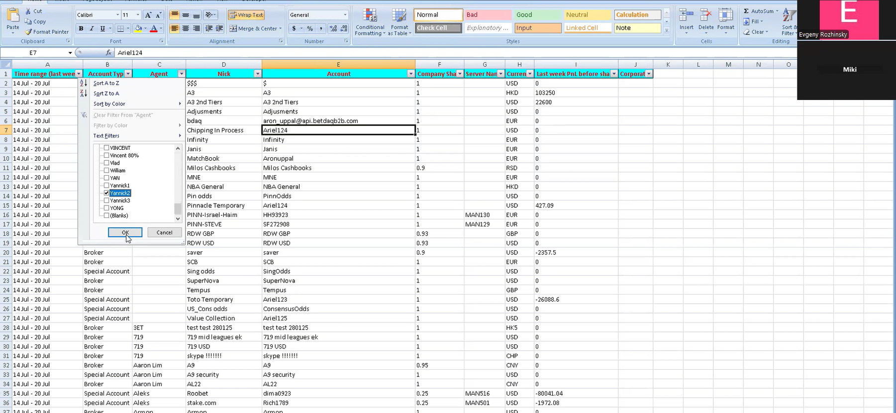
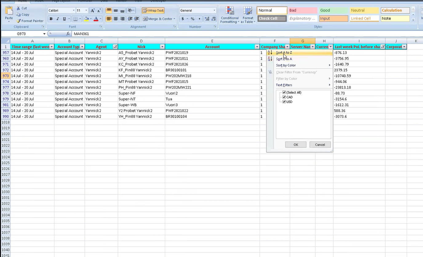
Remove all "0" on last week PnL before share column.
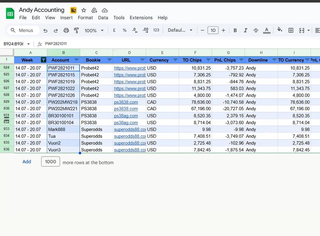
9
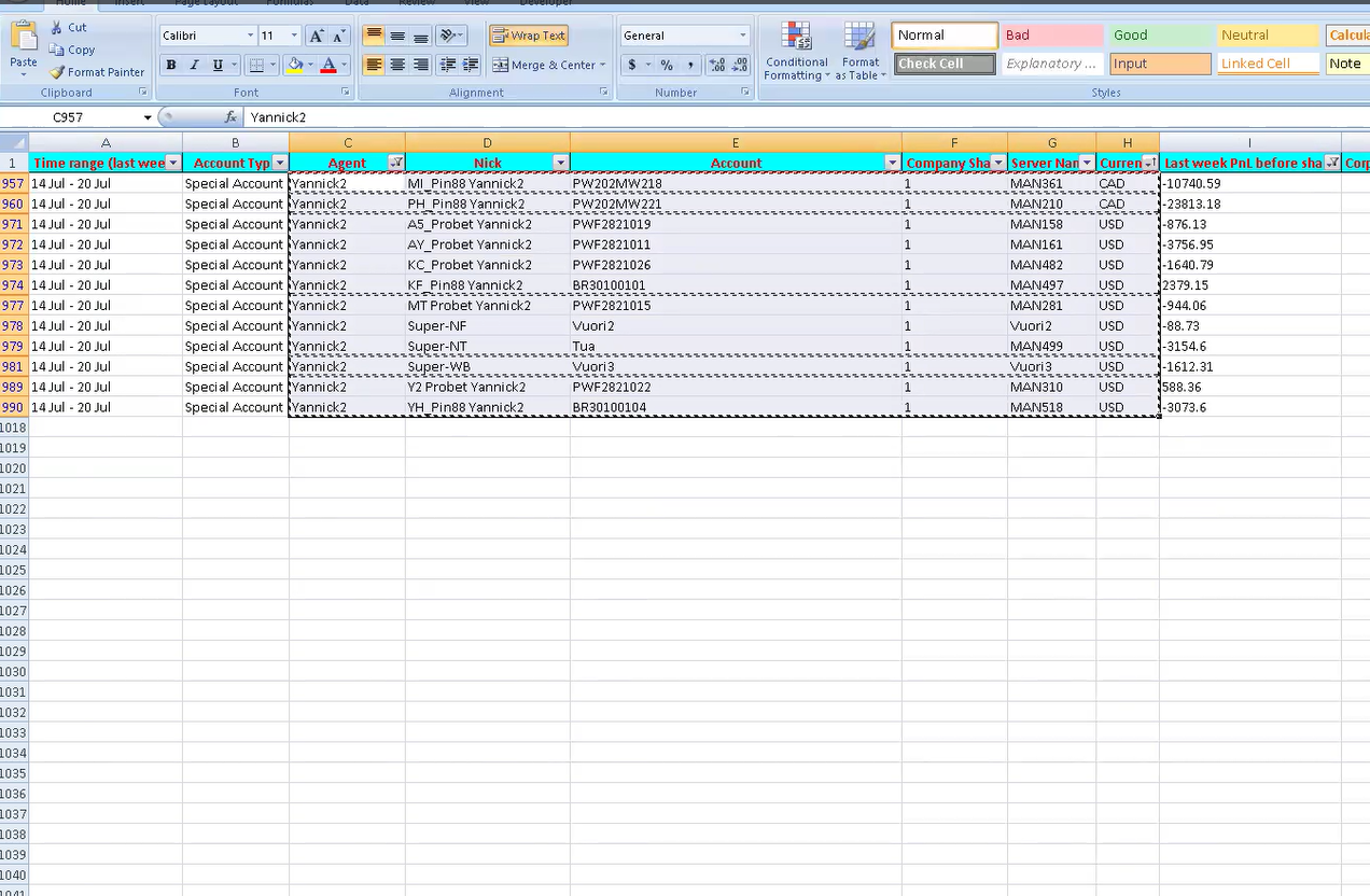
There are revevent accounts then sort A to Z by currency column.
10
Take Yannaick2 data to the weekly PnL file. Copy from Agent to Currency.
11
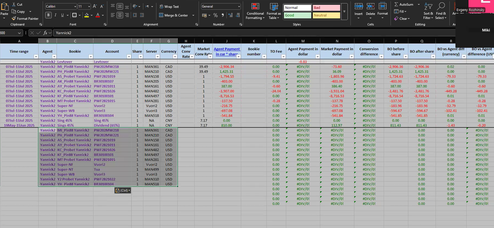
Paste them in the table (weekly PnL file).
12
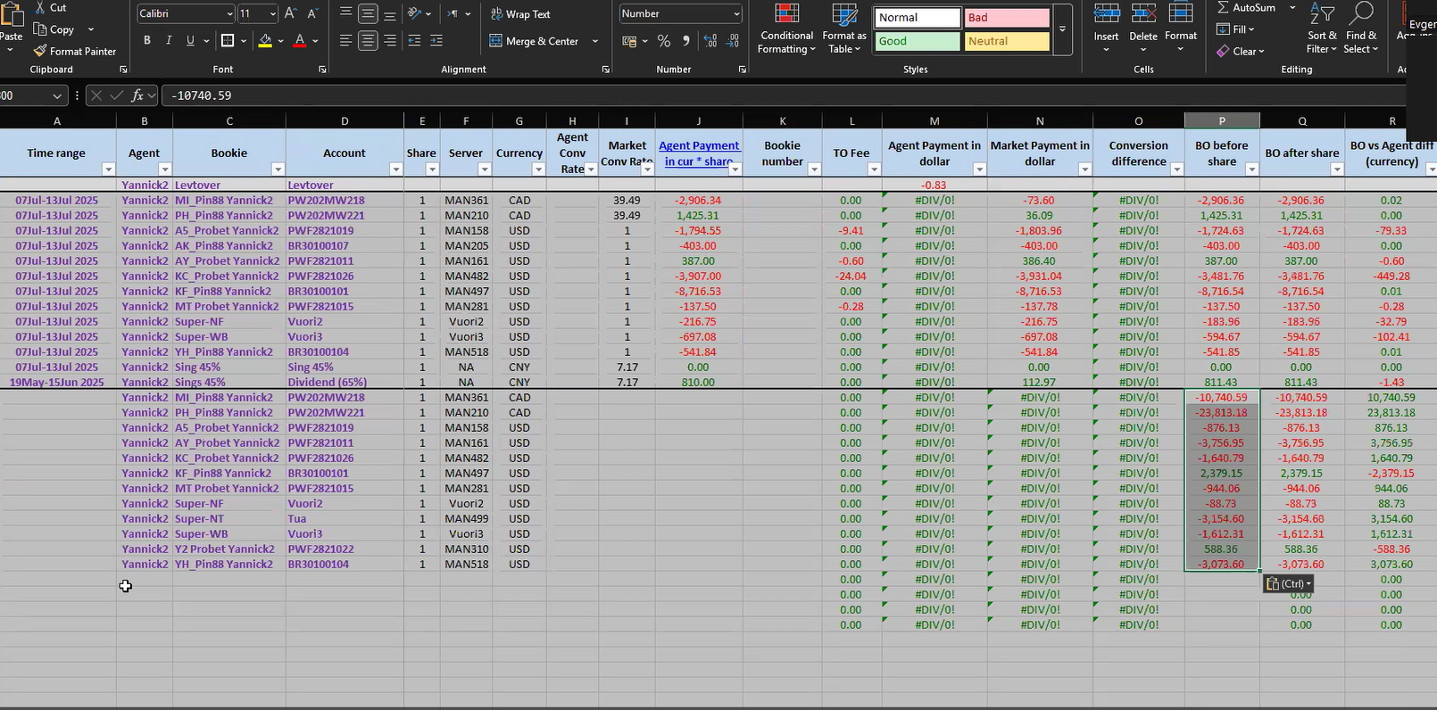
Then do the same as "last week PnL before share" column.
13
Copy sing and patse on the bottom.
14
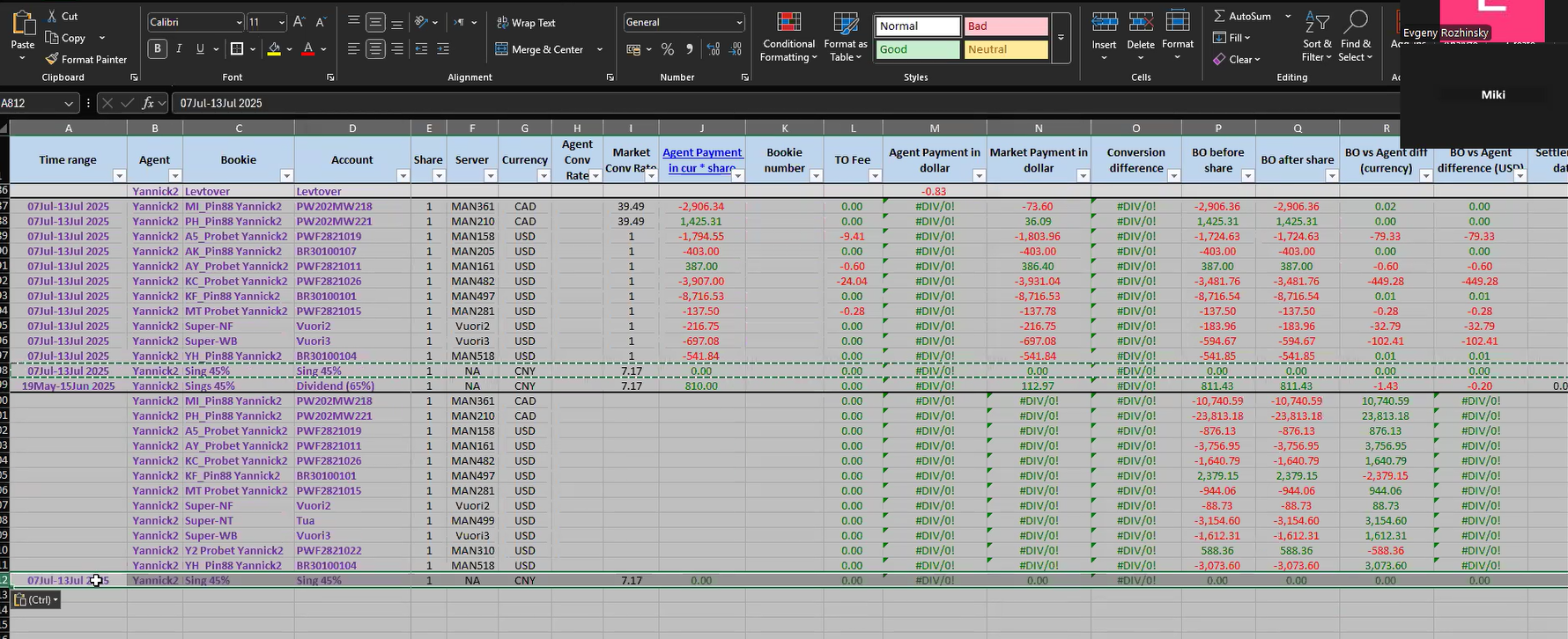
Add the time range (last week) into the excel.
15
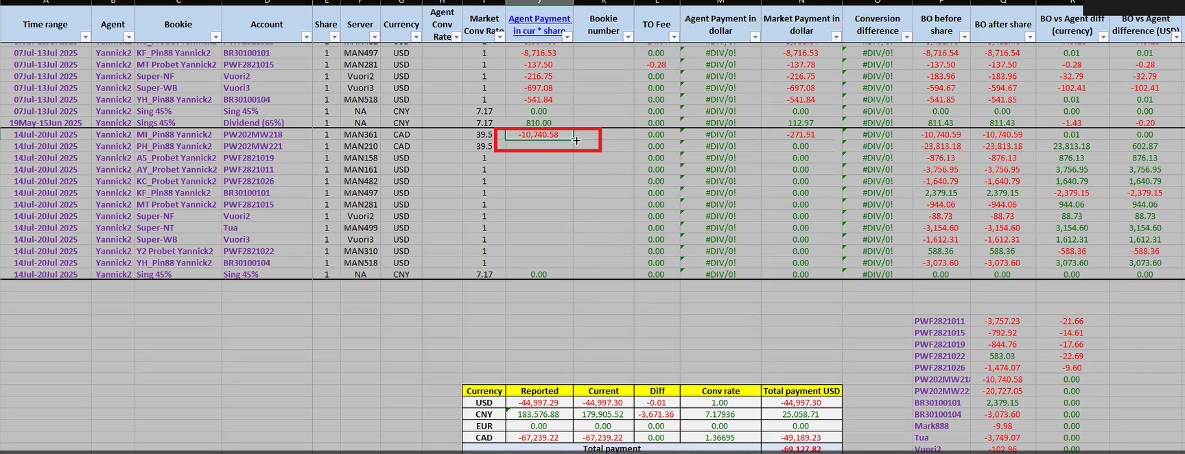
Add number on "market conversion rate" column by USD=1, CAD=1.38412 and CNY=7.17 Check rate again .
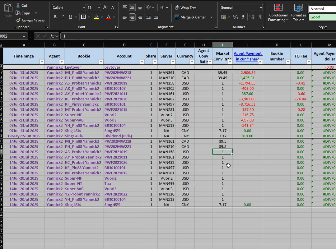
16
Click on "Agent payment" column to open the agent's spreadsheet.
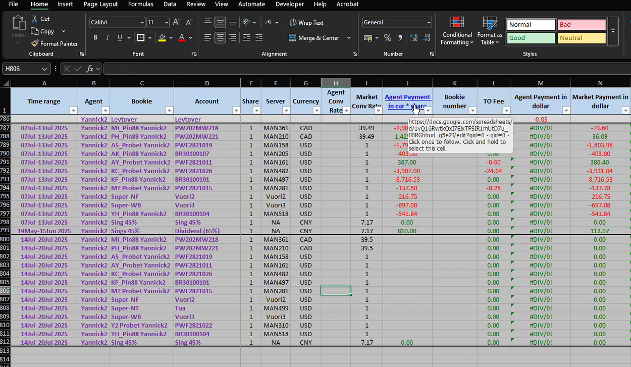
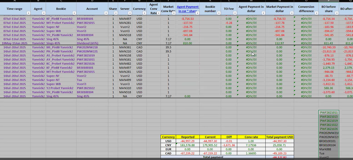
17
Filter by the time range (last week).
18
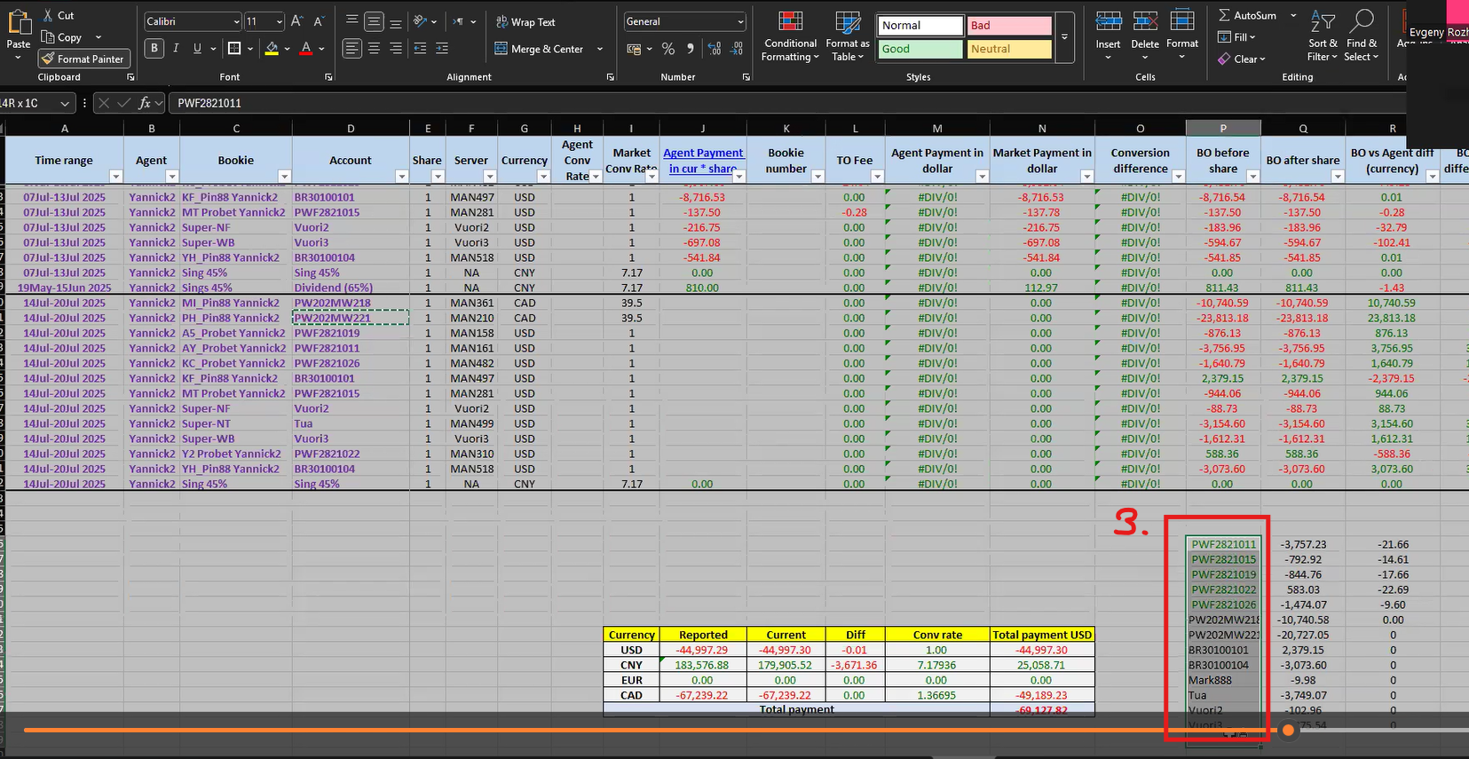
Copy account names from the agent spreadsheet to our excel.
19
And paste in the our excel as shown in the screen shot.
20
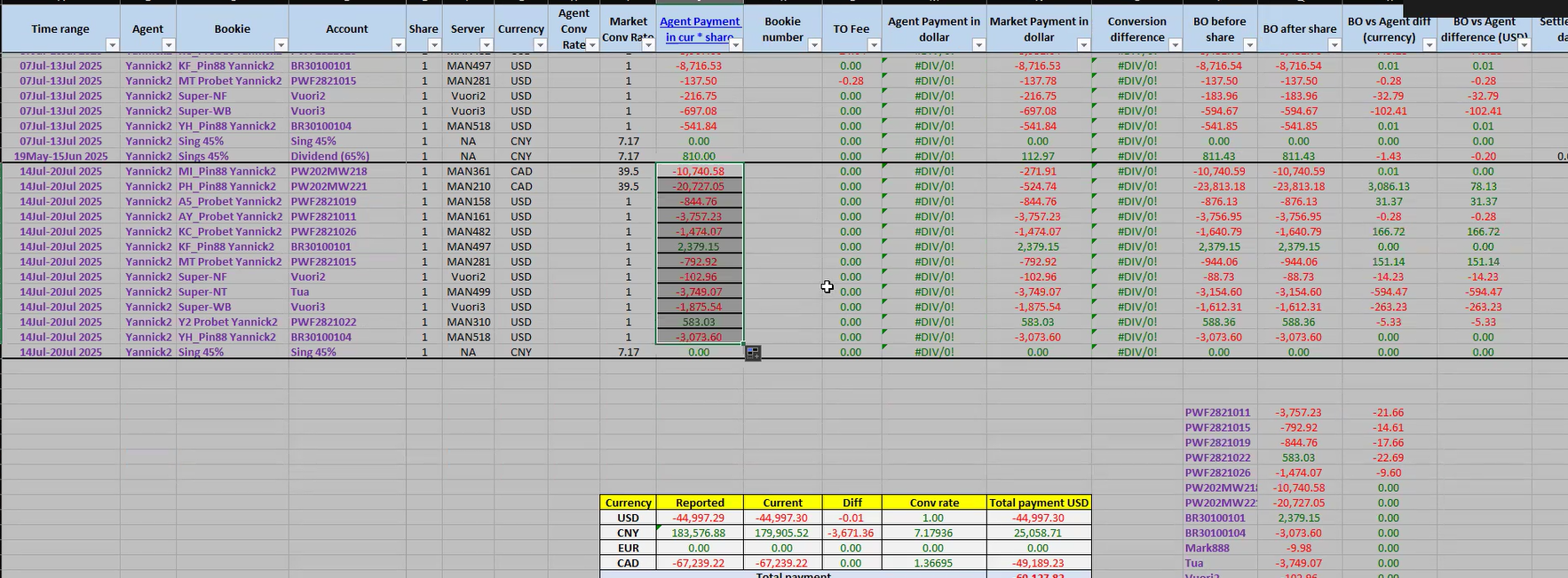
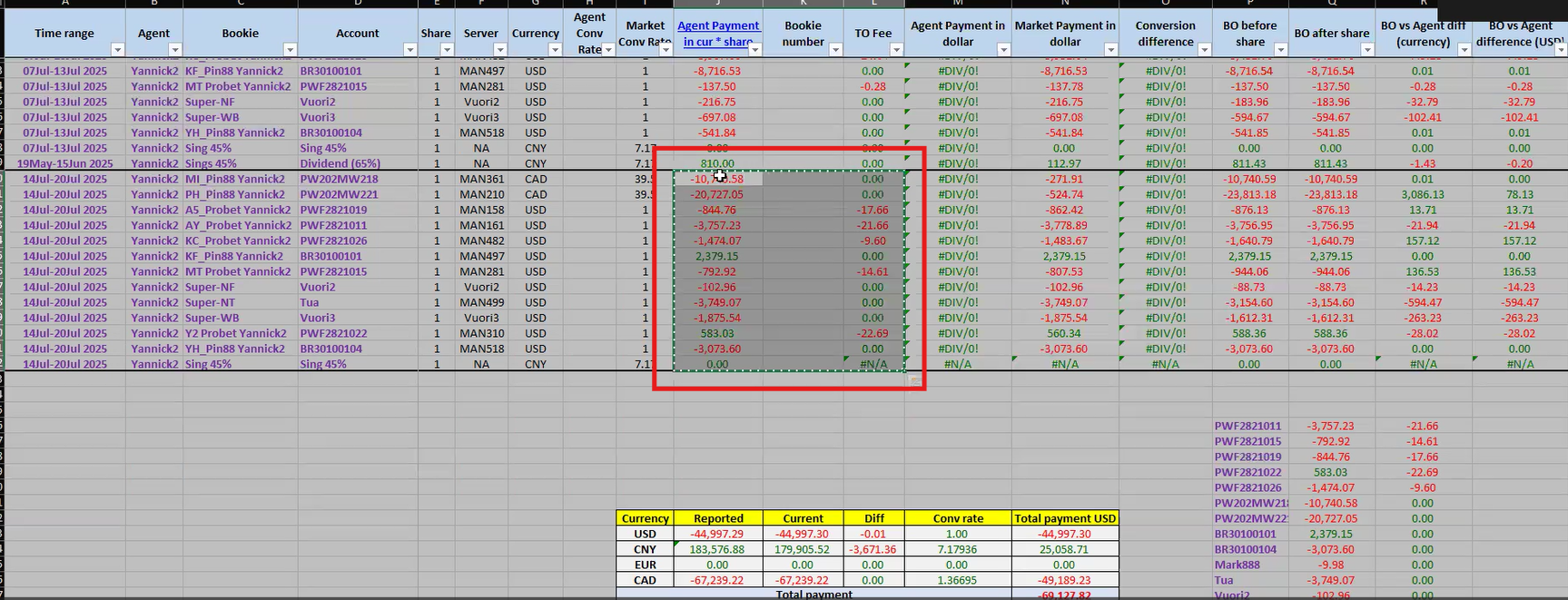
Then copy PnL Currency (PnL after share) and TO Fee from the agent's spreadsheet.
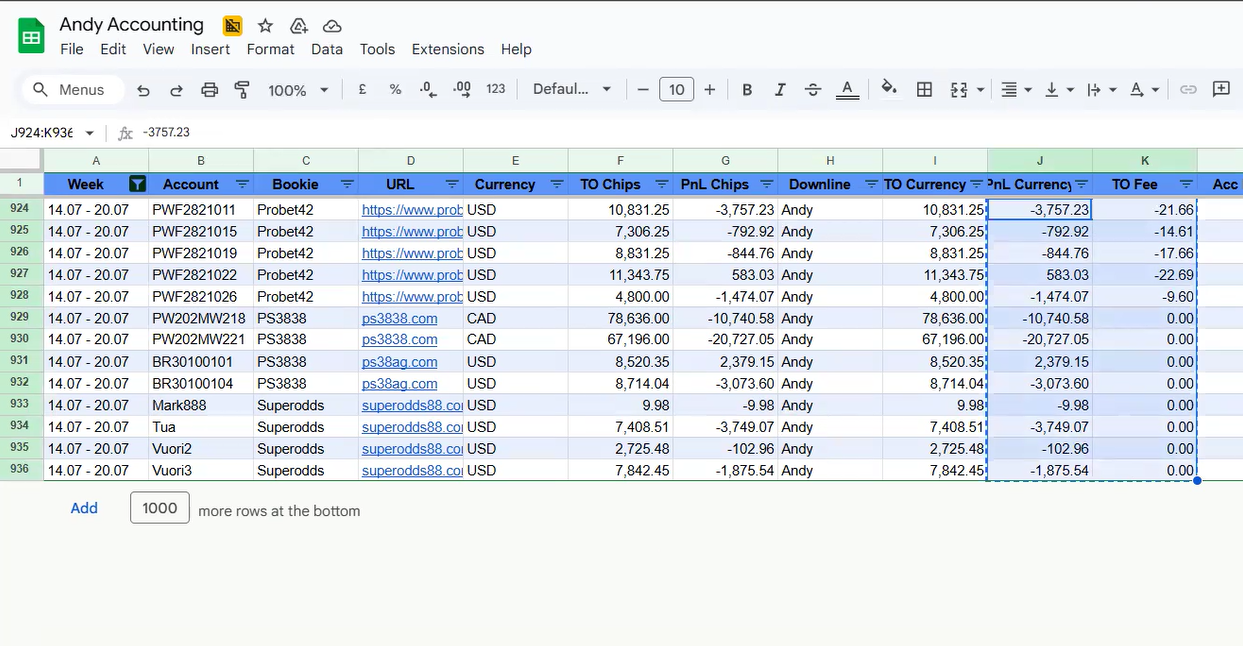
21
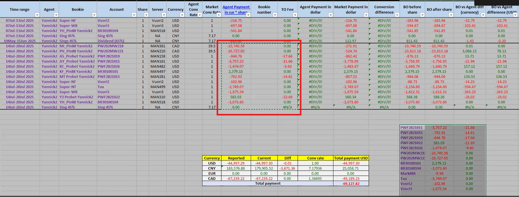
And paste them in the our excel.
22
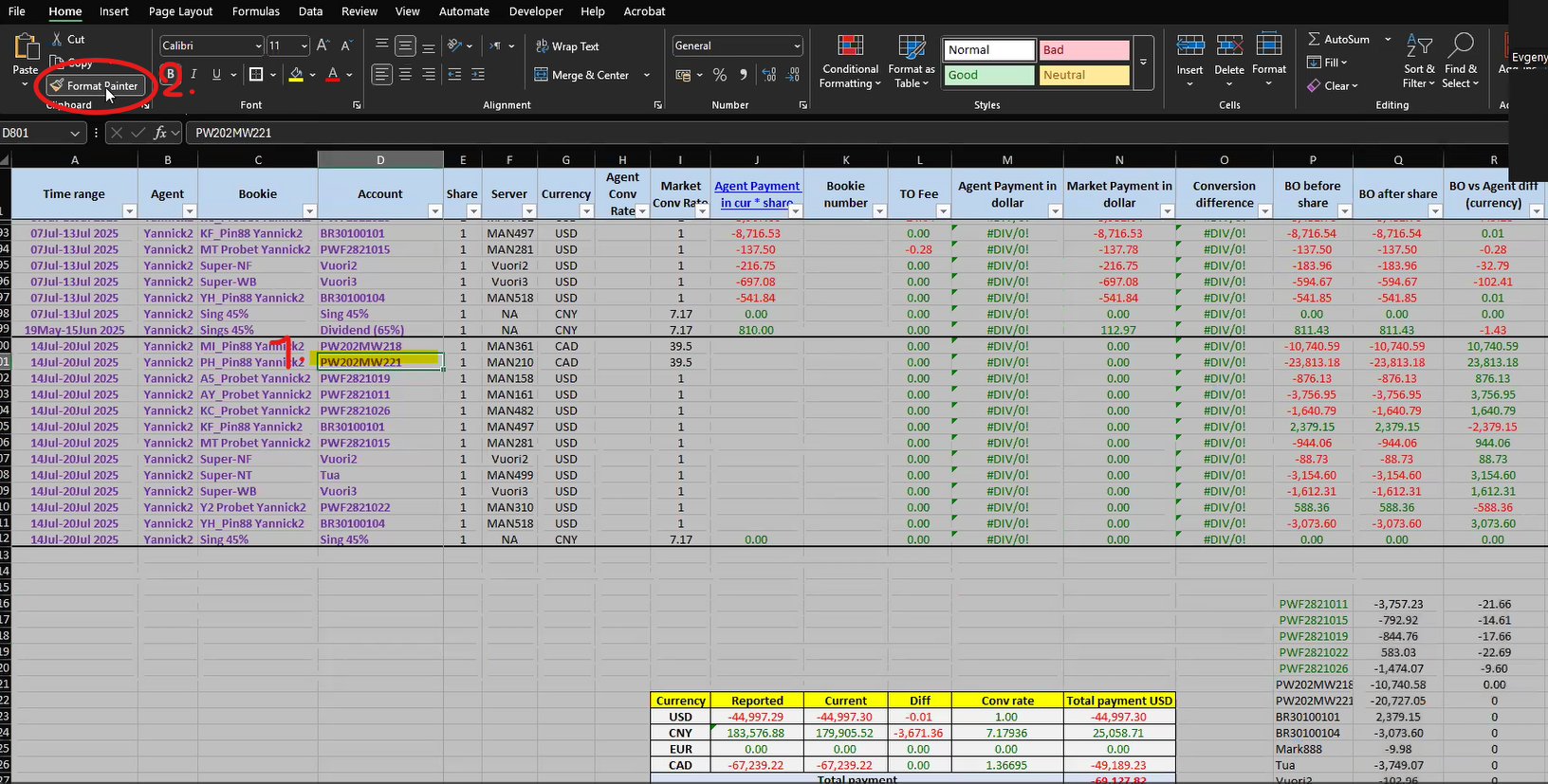
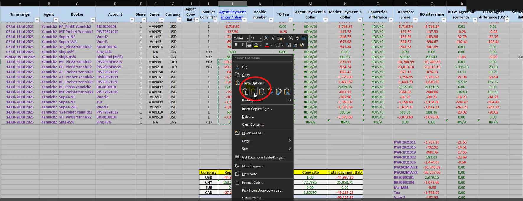
Set the data format to match them in the table. 1. Select the account name in the main data. (Account column) 2. Click Format Painter.
23
3. Select all the account names to automatically apply the formatting
24
We will get both sets of data in the same format.
25
Follow the same steps as in steps 22-24 for the PnL currency and TO fee data.
26
We will get both sets of data in the same format.
27
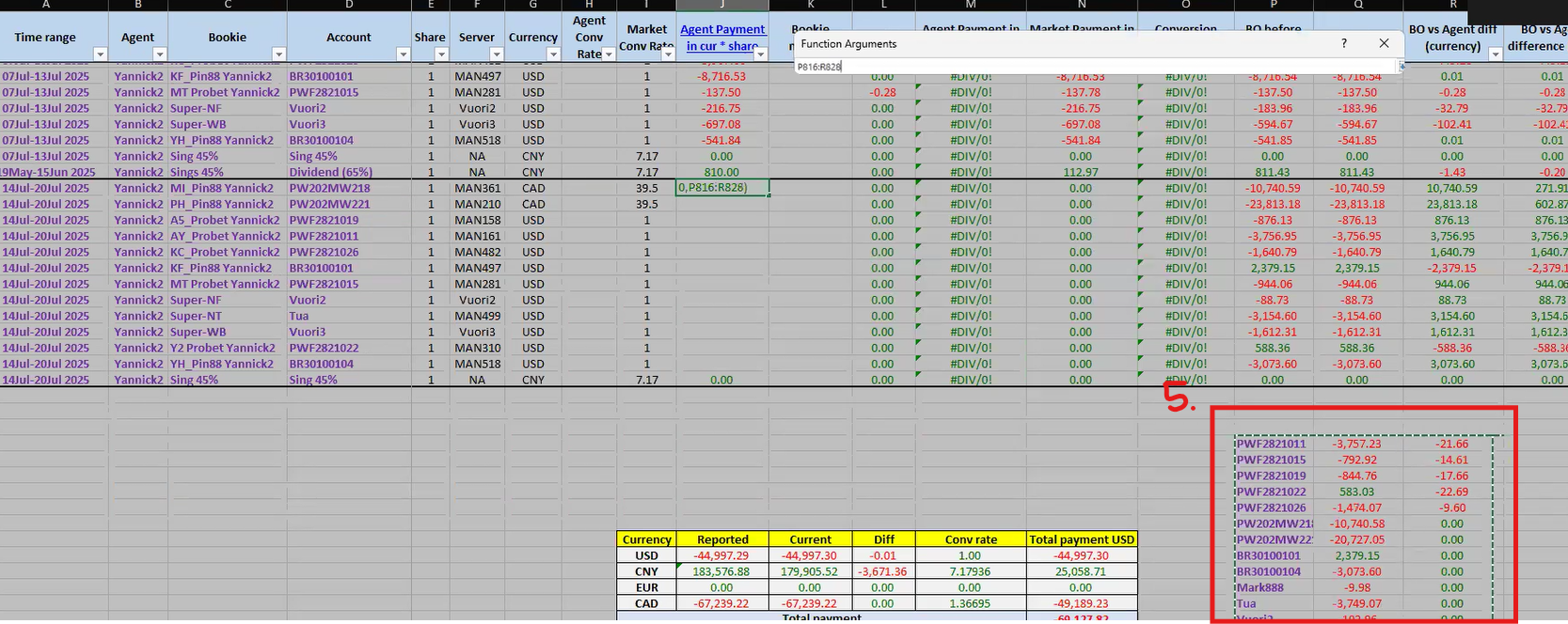
Add them to the main data in "Agent Payment" column. 1. select the table. 2. Click function 3. Select Vlookup.
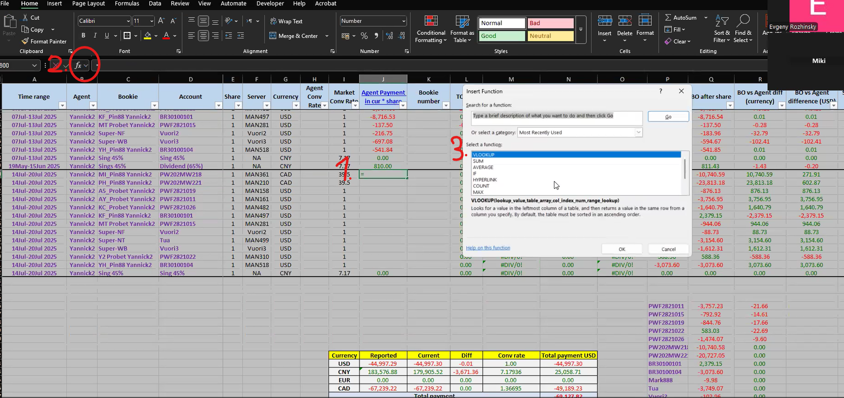
28
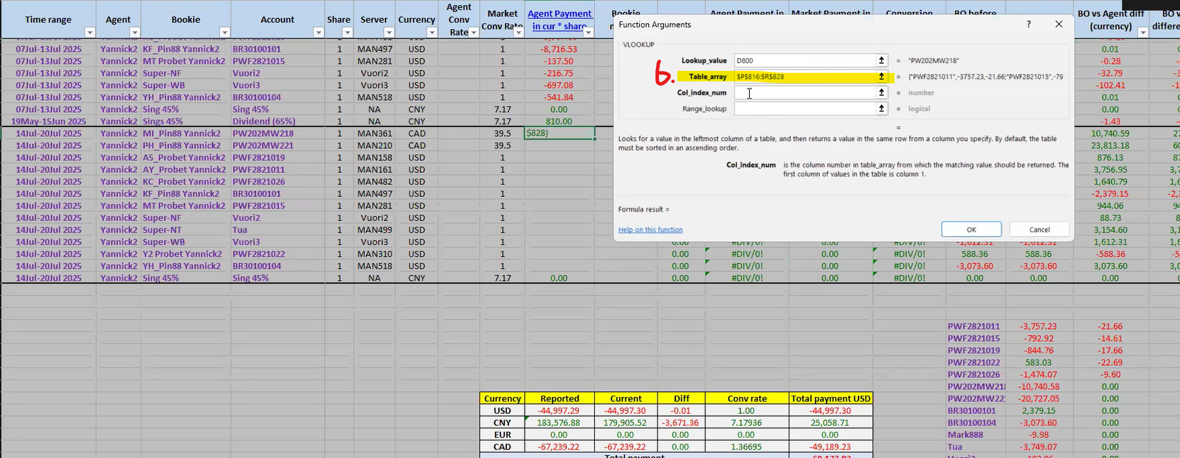
Seclect the user name in Lookup_value.
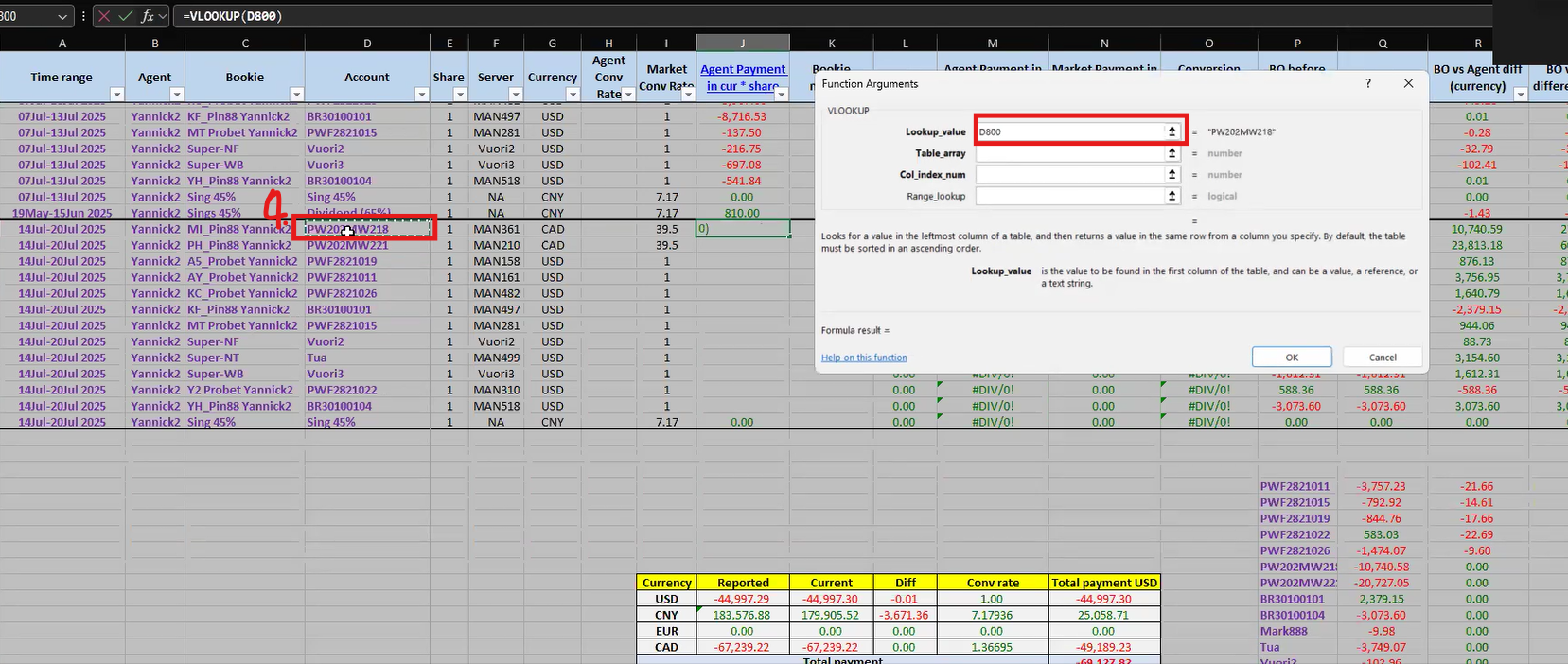
29
Select the data range to input to Table_array.
30
Then add "$" to lock the data range. ($letter$number:$letter$number)
31
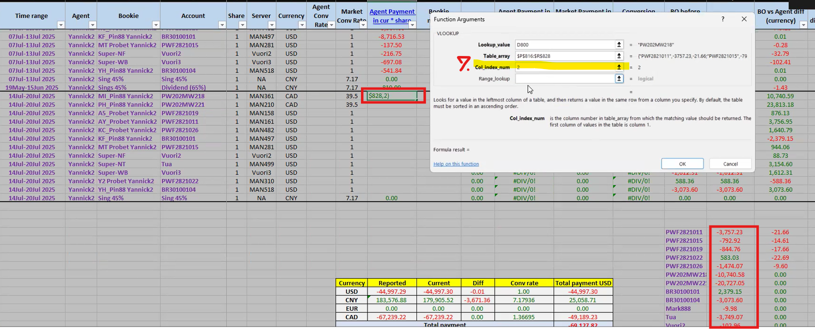
Add "2" on Col_index_num that means the PnL current values will be matched with the username in the main data.
32
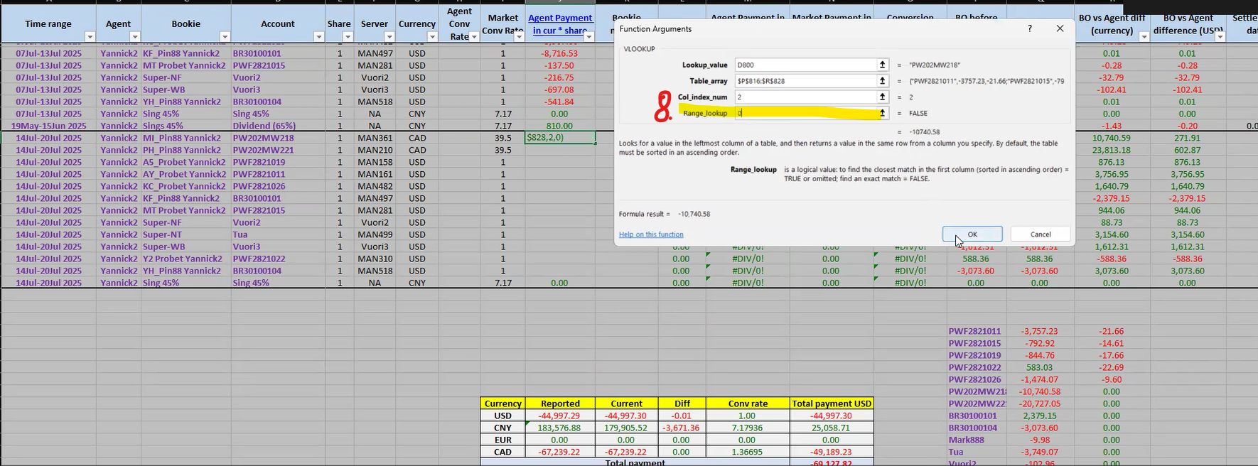
Add "0" on Range_lookup to match exact value.
33
We will get the number that match with the username.
34
Drag the format down.
35
Follow steps 27-34 with "TO Fee" but change to be number 3.
36
Make sure all the data in the table follows the same format by using format painter.
37
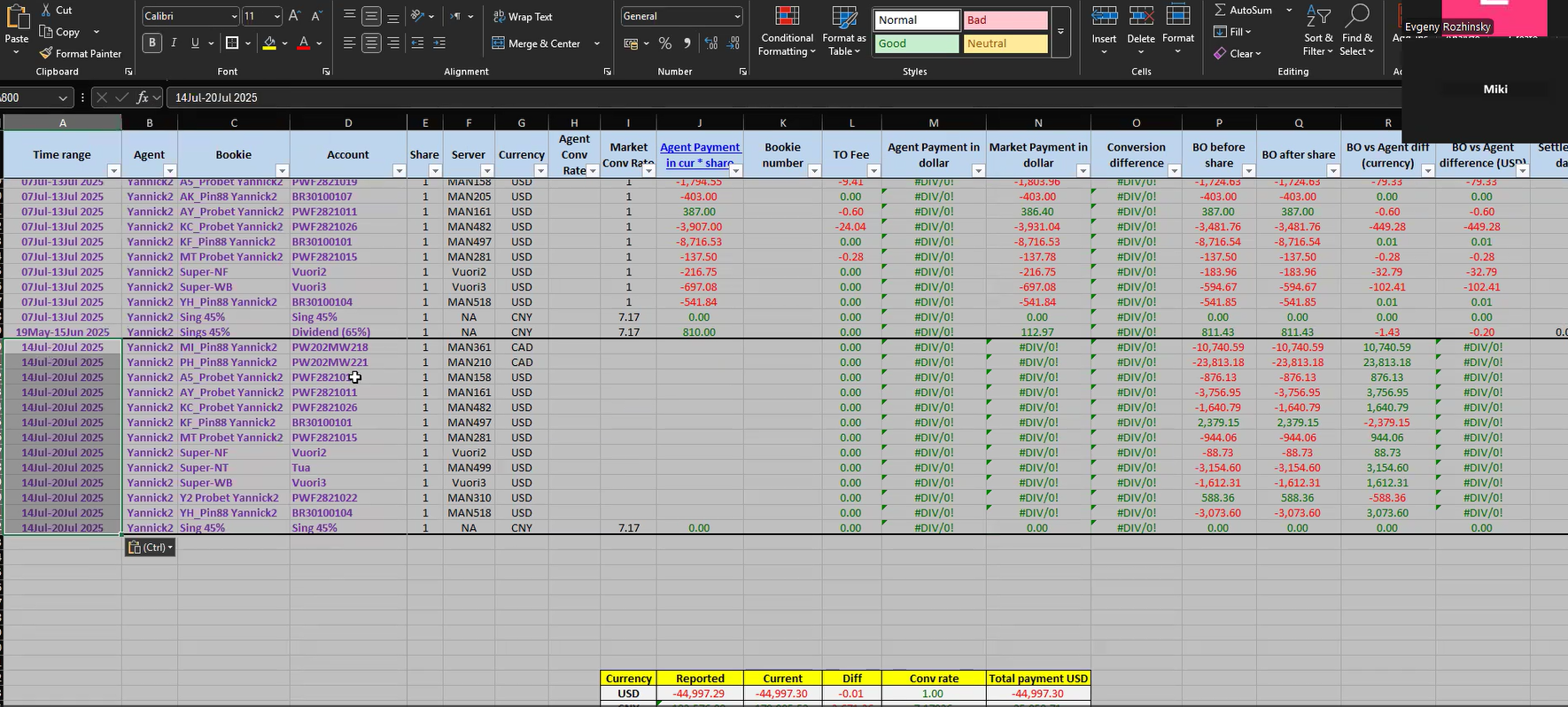
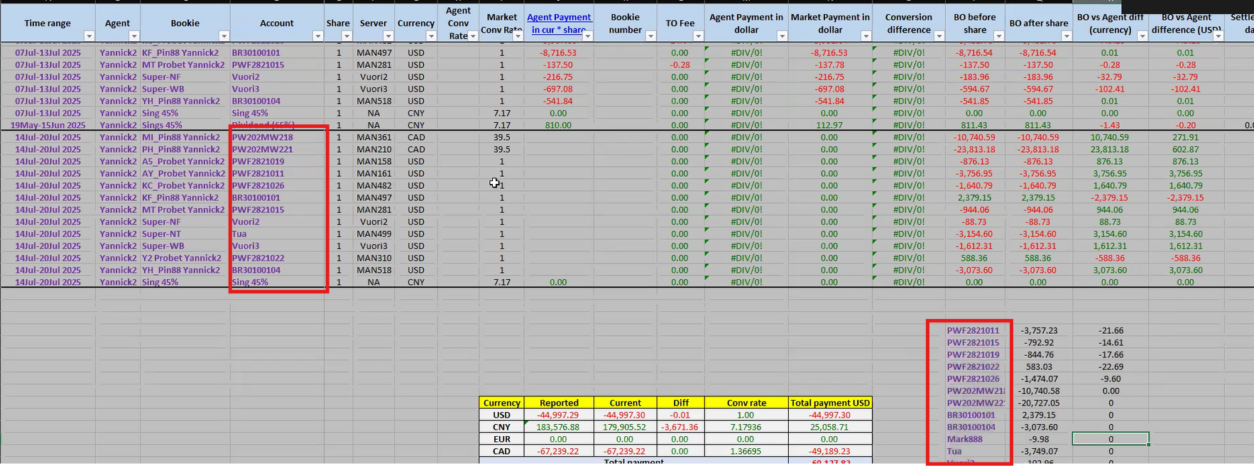
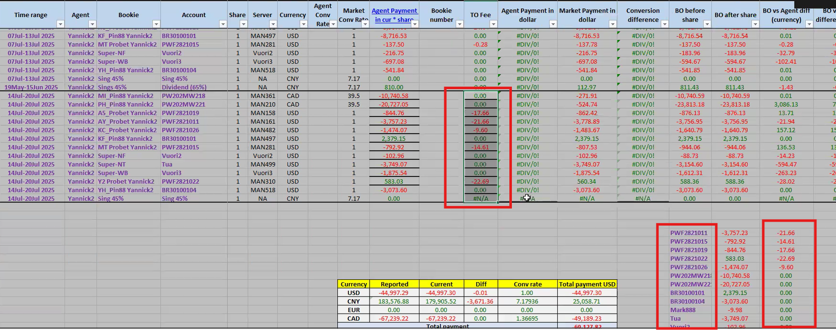
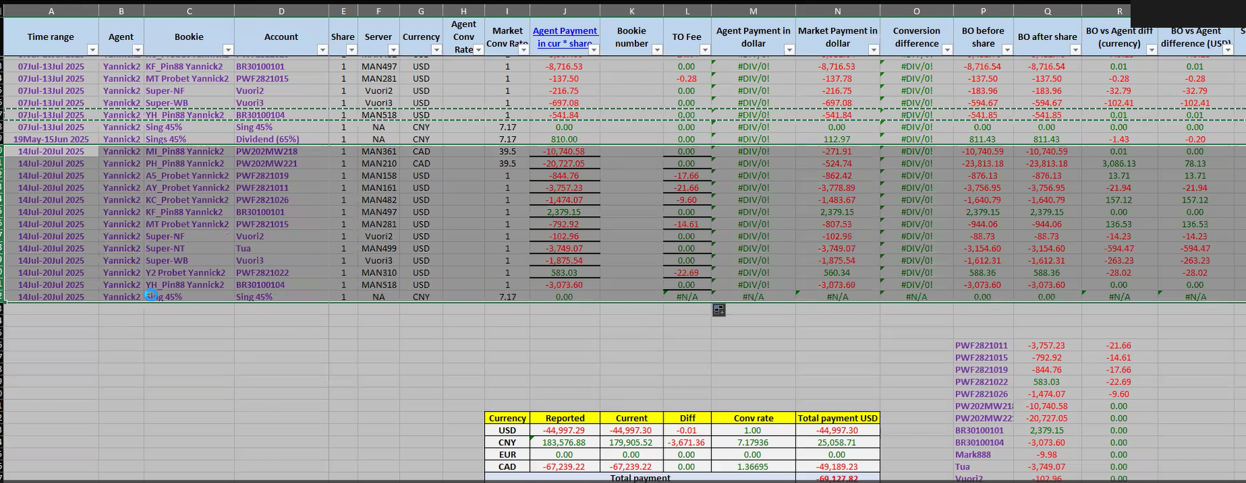
Copy PnL and TO fee data in the main data.
38
And paste it as values to get rid from the formula.
39
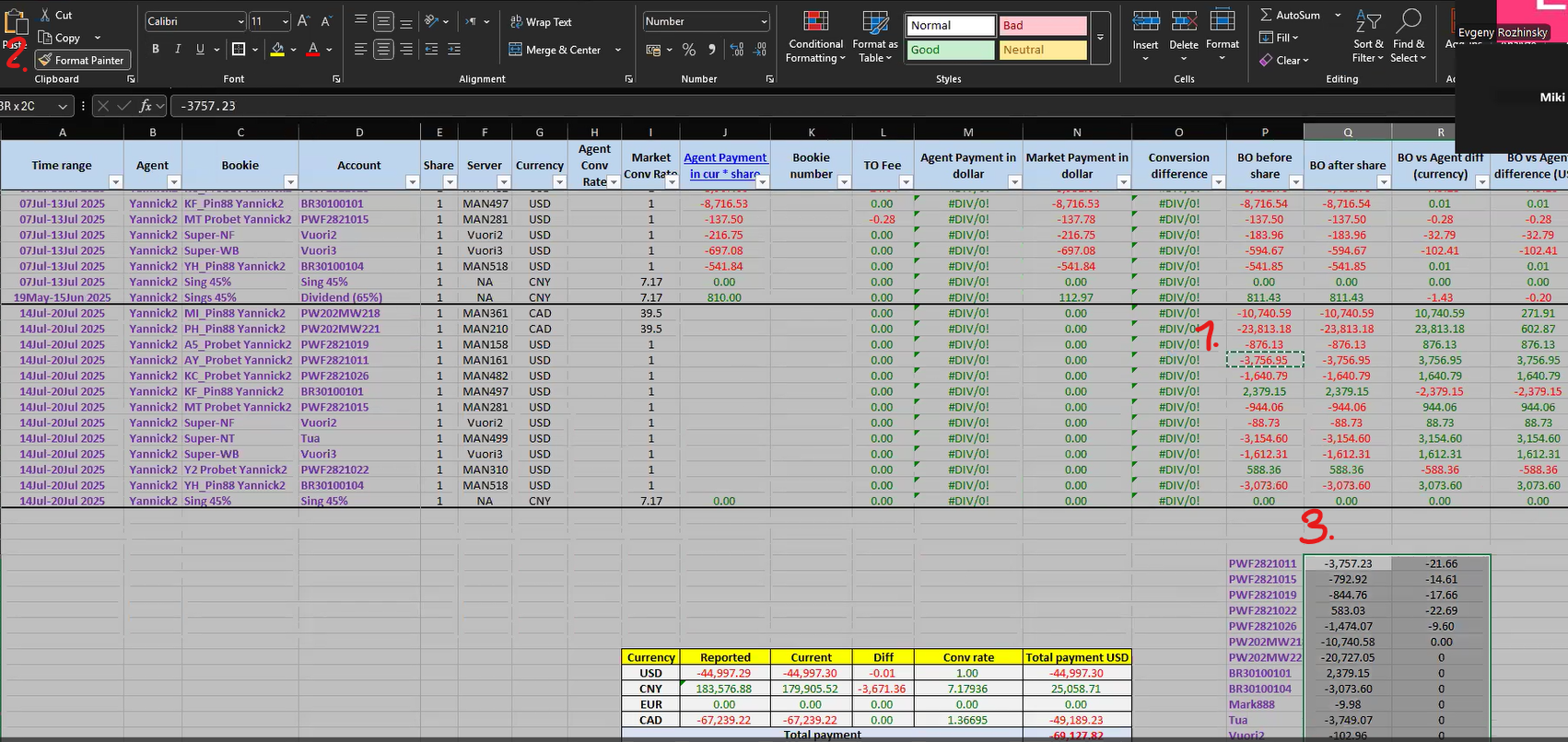
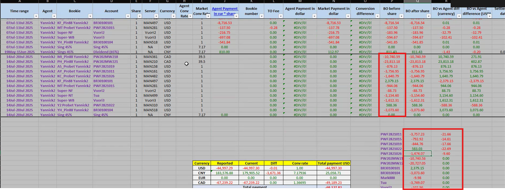
40
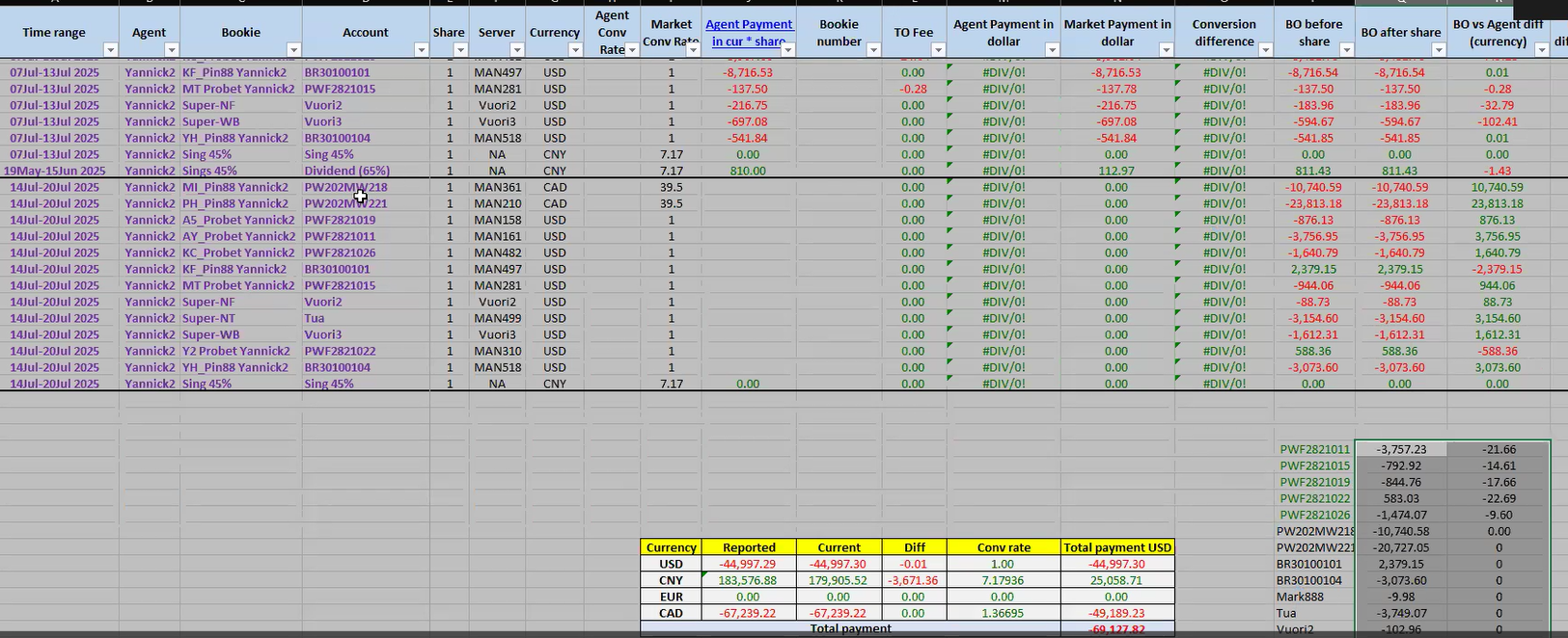
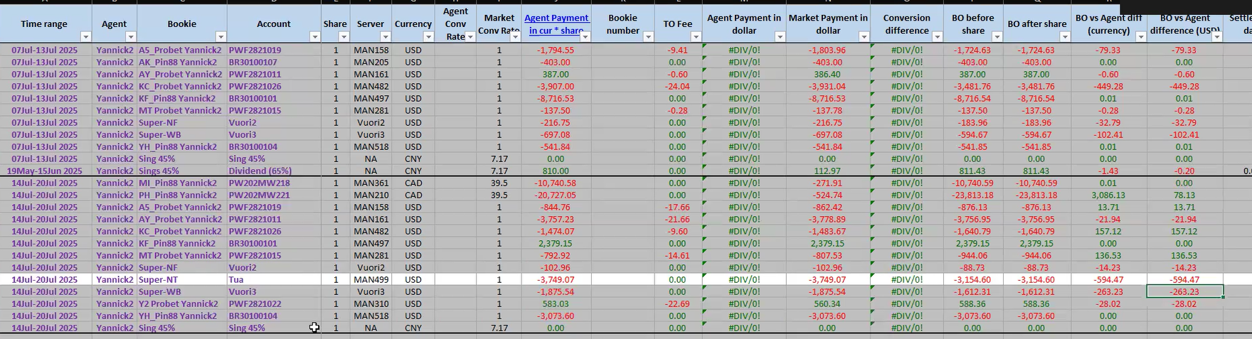
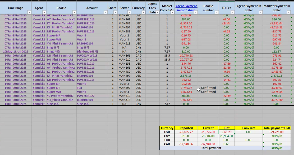
Check on BO & Agent different (USD) column. If the red - the mismatch is against us. If the green - the mismatch is in our favour.
Confirm the balance
41
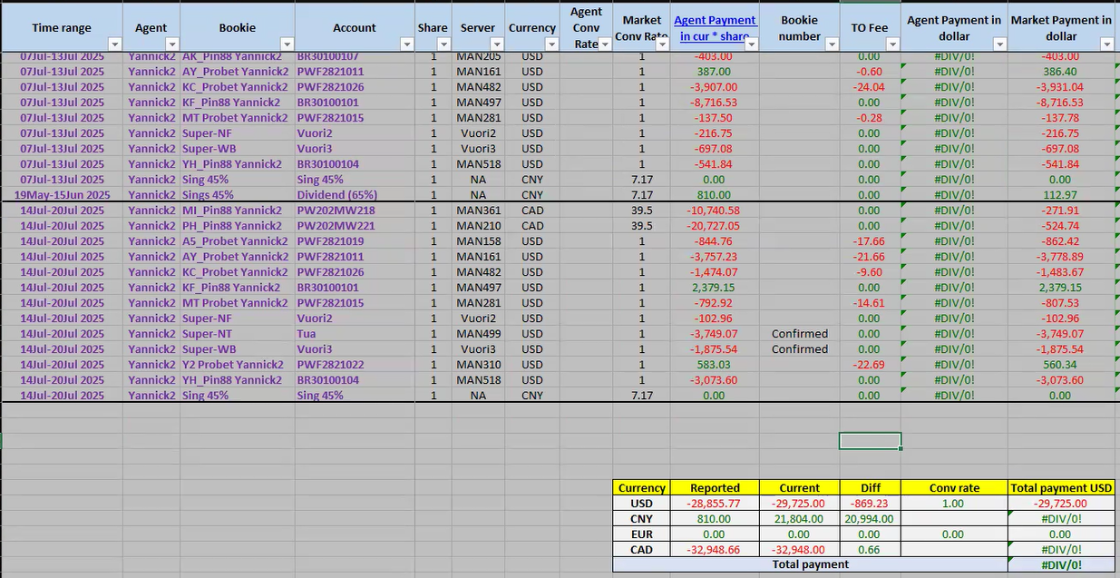
Prepare the table on weely PnL file to fill the new number.
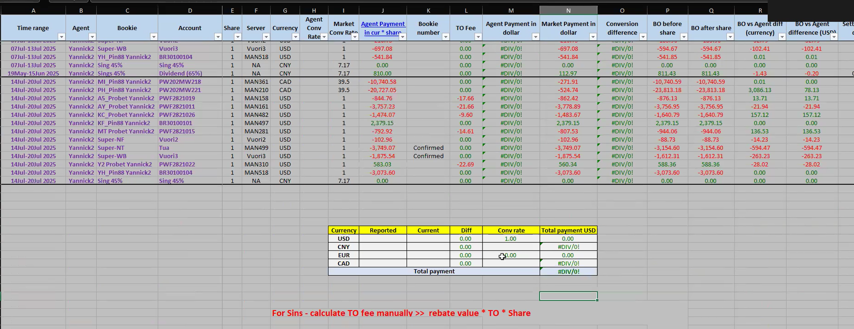
42
Add up all the USD amounts in the "Reported" column.
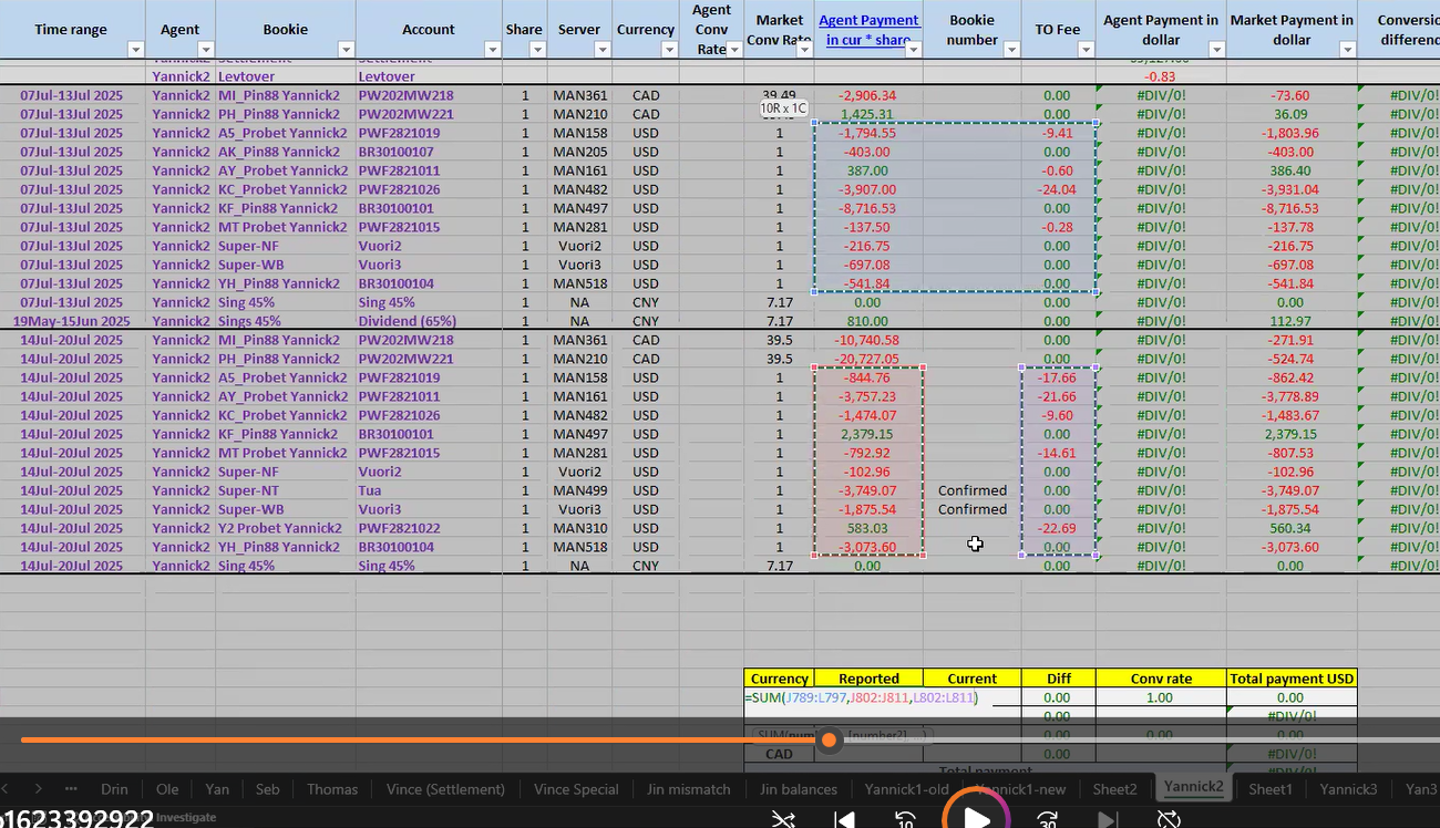
43
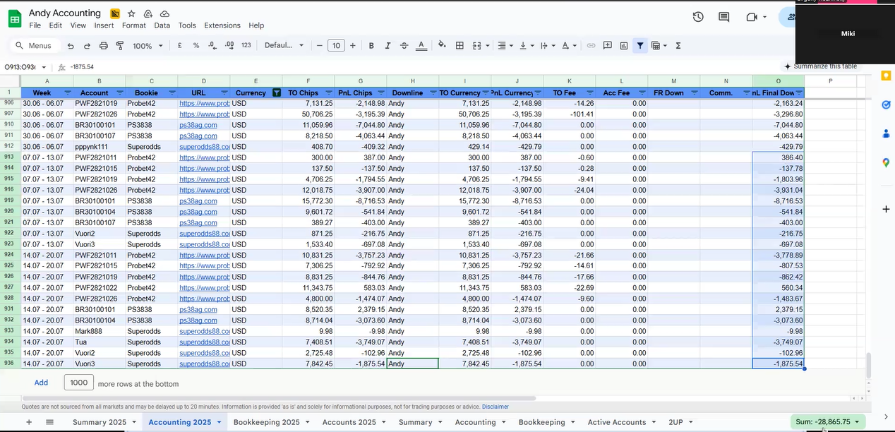
Open the agent file (summary 2025 sheet).
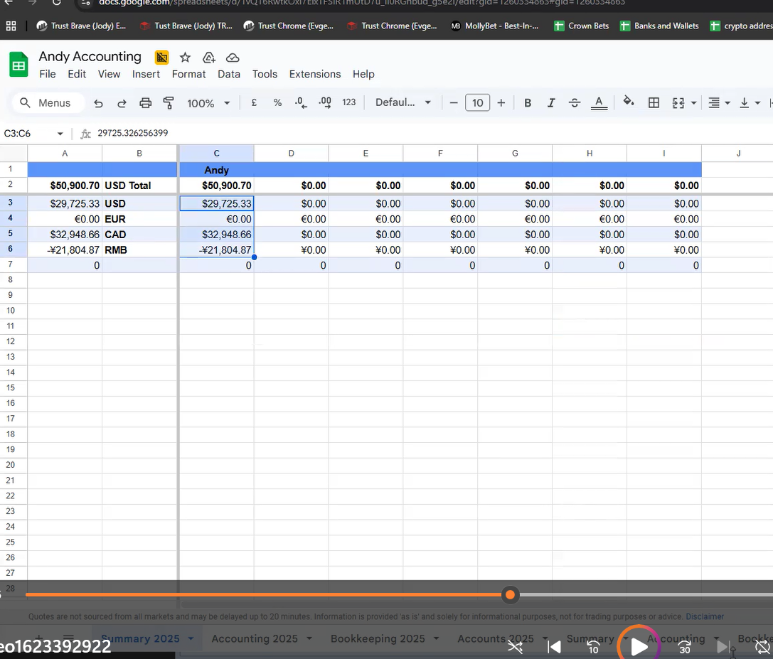
44
Take the number from the agent spreadsheet into our excel in the "Current" column.
45
Follow steps 42-44, CNY, EUR and CAD untill all are done.
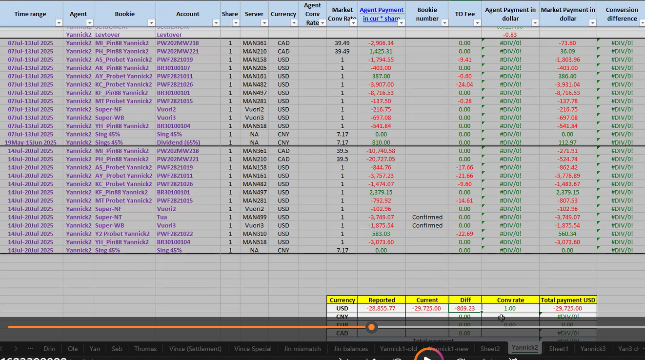
46
Check in the "Diff" column. If there are any discrepancies, find the cause by going back and checking the statement page from agent again.
47
Filter by date and currency, then check the total again.
48
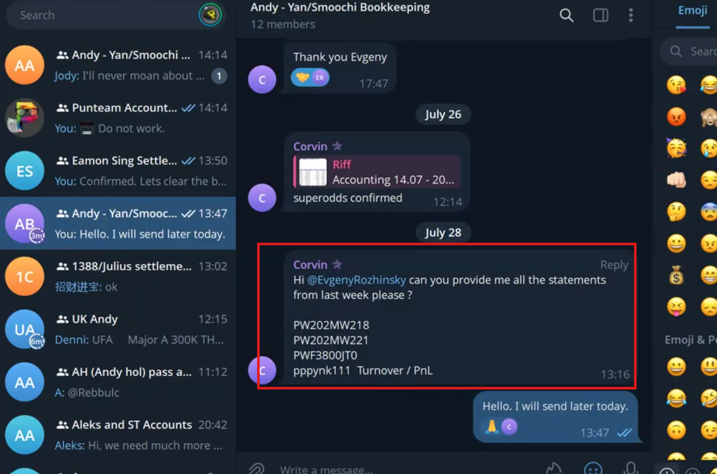
If it still mismatches, report it to the agent in the chat group. And wait for the agent to check and correct it if there is an error.

They request us to send the stagement of the accounts
49
50
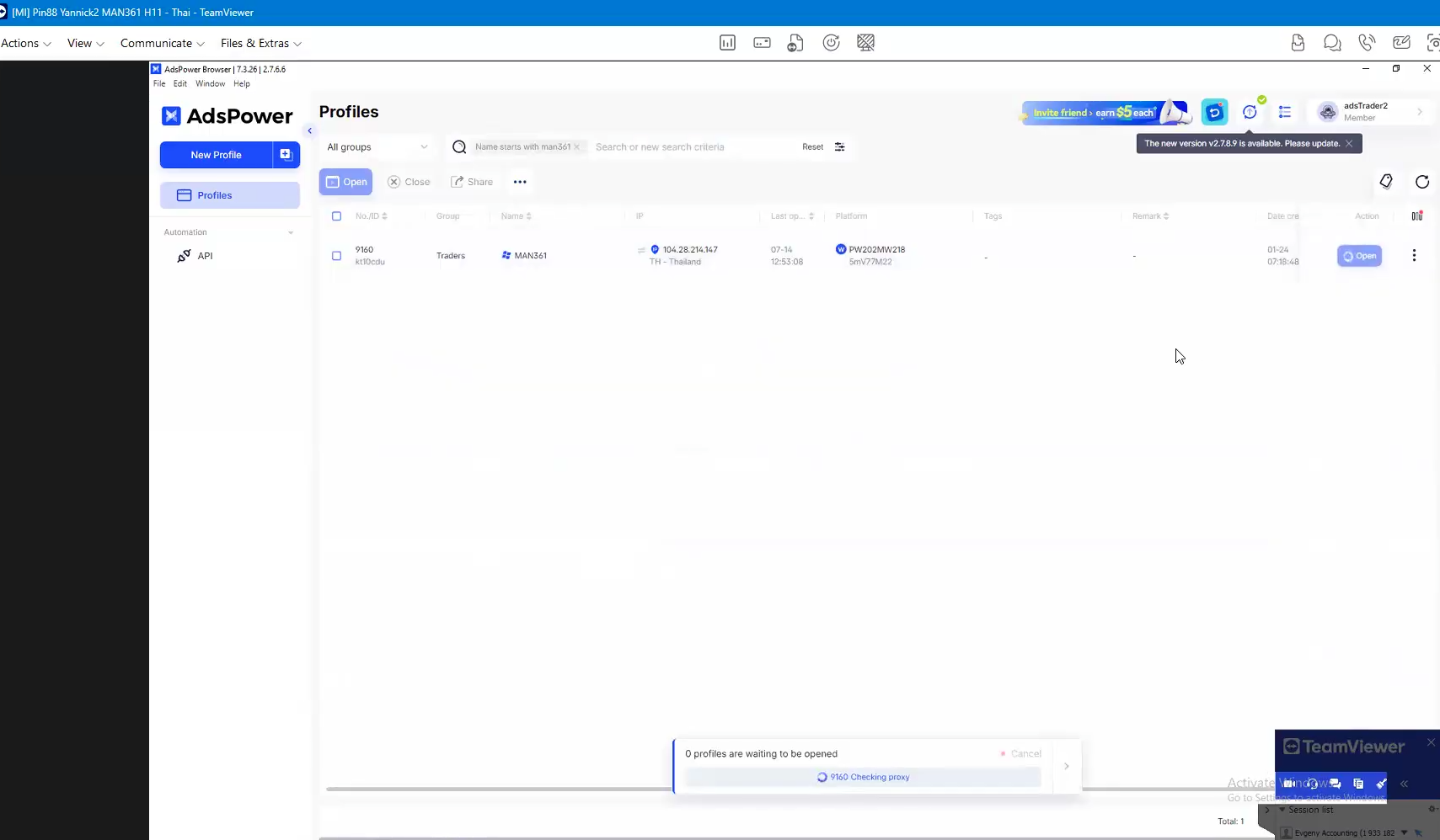
Go to server on that account.
51
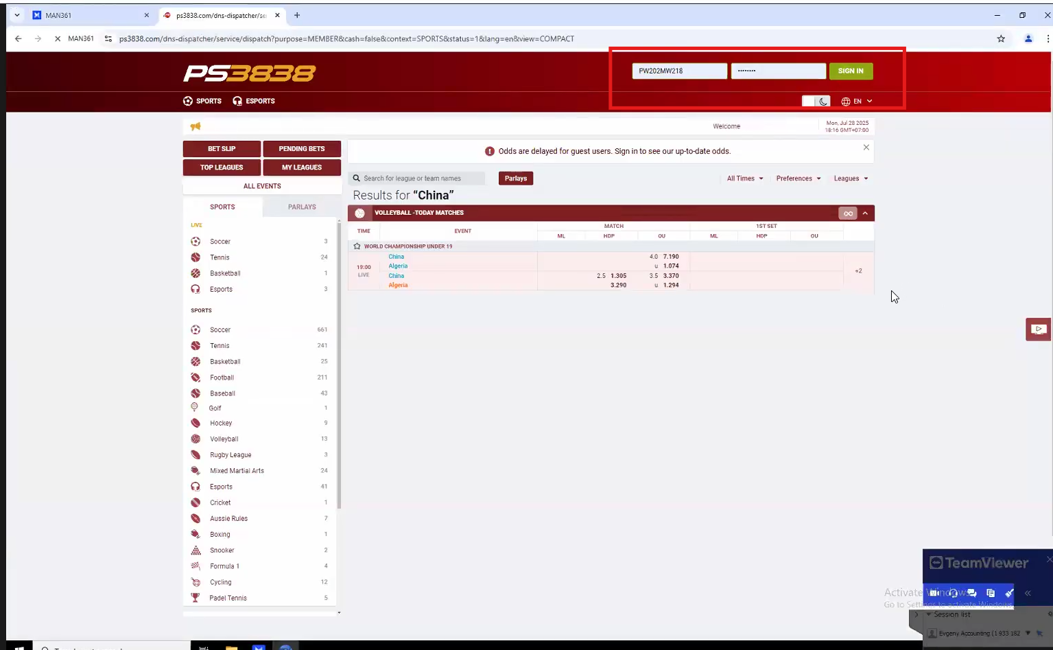
Sign in.
52
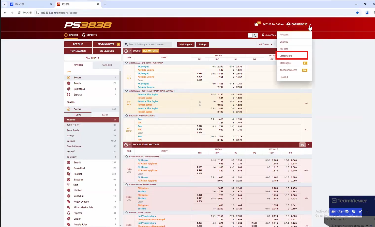
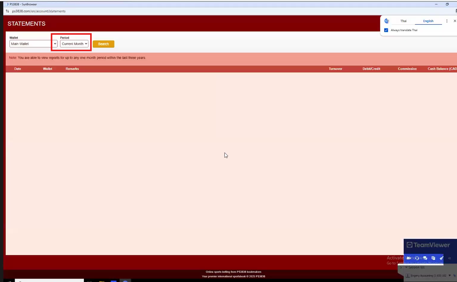
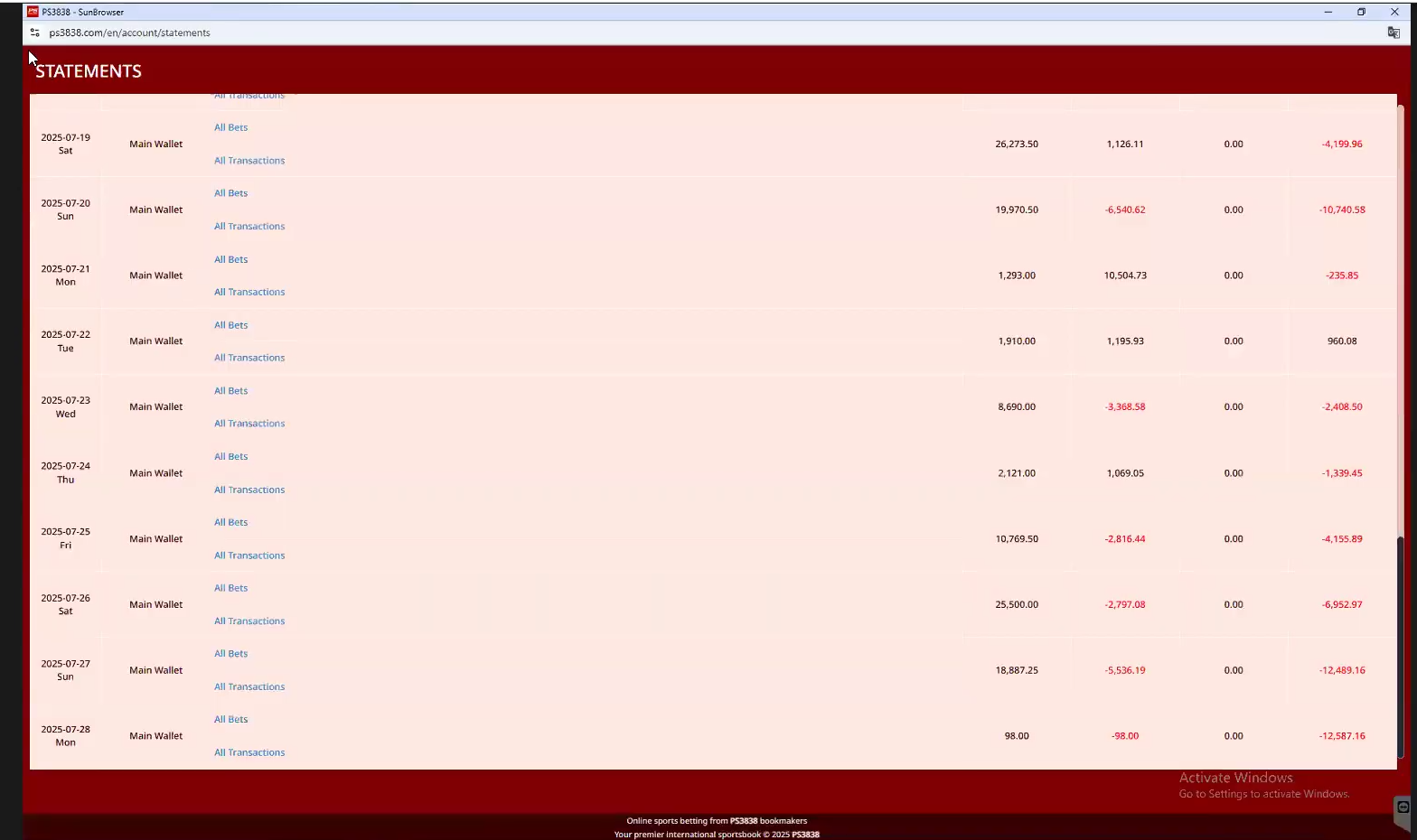
Go to statement page.
53
54
Make the screenshot and send to the yannick2 group.
55