Optimizing Spreadsheet Data for PayPal Transactions

In this guide, we'll learn how to organize and match data from different spreadsheets to ensure consistency across columns. This process involves aligning categories such as type, date, and currency, and converting formulas into static values for easier manipulation. By the end, you'll be able to efficiently manage and sort your data, making it ready for further analysis or reporting.

Let's get started

I've placed a copy of the spreadsheet here to view the categories we're working with. I'll try to match the columns with the new data as closely as possible. I have a type column and a date column. There's only a start date, but I also have a completed date here, which I prefer because it serves as the post date. So, I'll use the completed date.

1

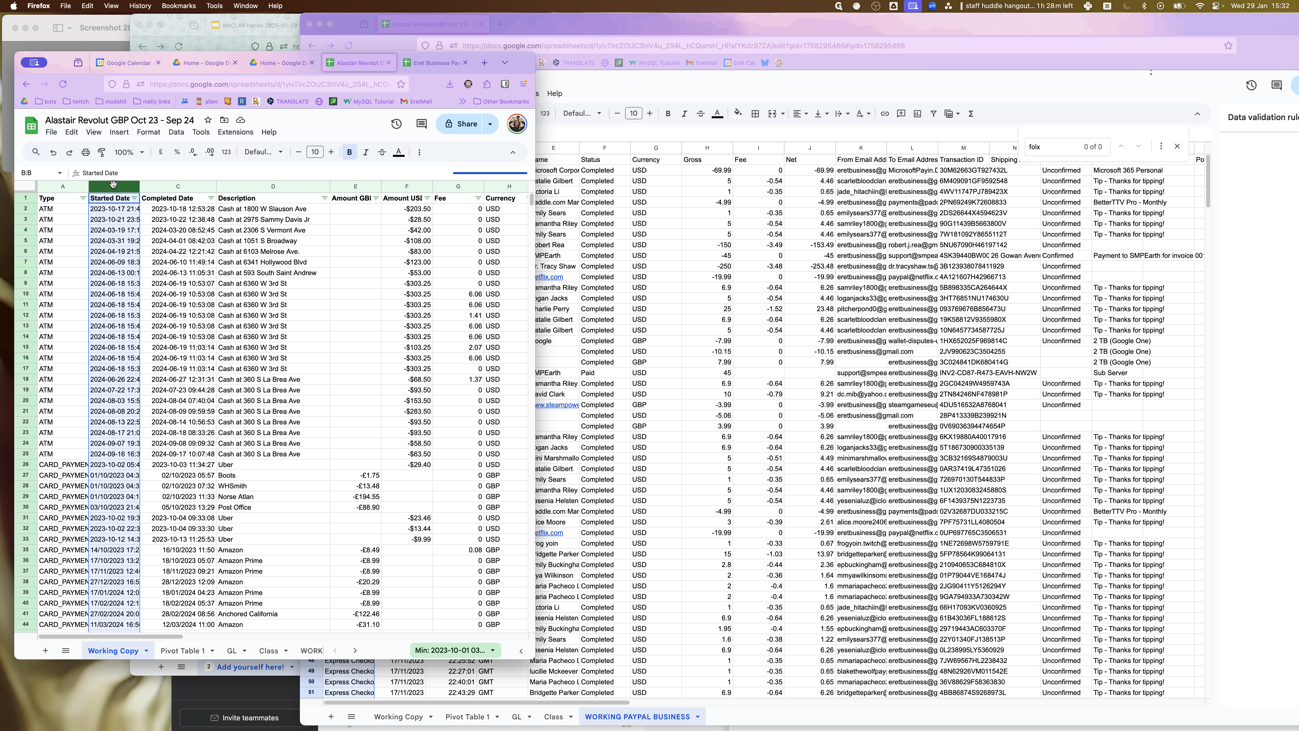
My date is the same. I don't need the time, so I can delete it. The description will be similar to PayPal's item title. In this case, PayPal is close to the name. So, I might use type, date, name, and then we have amounts in Great British Pounds. This part is interesting because we have two elements mixed into one here.

Let's focus on the column to the right, as that's how they came in through PayPal. Now, we'll use the formula: if E2 equals GBP, we'll take the net amount. If not, we'll display "none." We'll apply the same logic for USD by changing the formula to check if E2 equals USD.

That's two, okay. Now we will copy that all the way down. We have these two things separated, which is great. Next, we want to lock them in, so I'll copy them and paste special values only. This way, it stops being a formula and becomes just values. Then, I can move it next to the name to match these two. I have fee and currency, so I'll go with fee and then currency. The state is completed, matching the status. Do I have a balance? Yes, I do, but I don't think we'll need that necessarily for this.

Let's say we want to keep some information on the side. Is my glitter still there? I'm not sure. Anyway, all good. Now we have everything where we want it. Let me move the balance column next to the status.

Yes, okay. Now we can copy everyone except for that, and I'll move my class and GL on the original sheet to the side. This way, when we place it here, we can have all the extra information at the bottom without any issues. If I insert one row below—wait, do I have a filter on? Is that why it's not letting me? Oh, I see.

Okay. Format the data and remove the filter. Now we have removed the filter. It should let me add—oh no, I made a mistake. Okay. Ta-da! There we go.

Ensure all your columns are aligned. Once they match, you can begin filtering and sorting. Repeat this process for all your accounts.